Loser-Take-All Elections in the United States Senate
As the legend goes, George Washington once compared the Senate to a “saucer,” cooling the passions of the House as a saucer does to tea (United States Congress 1993). The Senate was specifically designed to be slower than the House at reacting to polarizing stimuli. Yet the Senate is generally quicker to polarize than the House, as I documented in my master’s thesis (Morse 2021). Congress began heating up considerably in the 1990s, when Republicans adopted a more uniform right-wing ideology and won a large wave of seats in both chambers. Many representatives in the House moved up to the Senate, which Theriault and Rohde (2011) found had a significant effect on polarizing the Senate. These scholars and most others generally take this to mean that polarization in the House seeped into the Senate.
This chapter offers a different interpretation of the dynamic between House and Senate polarization. The fact that the Senate became more polarized as more House members moved to the Senate does not mean the House is polarizing the Senate. Republican senators maintained a relatively steady ideological distribution throughout the 1990s; they just grew in number, especially from states that are systematically overrepresented in the Senate but not in the House. The more extreme wing of the party was a much smaller force in the House, but moving to the Senate gave these members a much larger platform. In the modern political environment, the Senate does not cool the passions of the House; it merely amplifies passions that the House keeps in check via equitable representation.
I argue that much of the polarization, democratic breakdown, and rising inequality of the last half century can be traced to the Senate, particularly to its extreme malapportionment.1 The Senate filibuster has been analyzed extensively by political scientists, but the effects of its malapportionment are more difficult to study empirically and thus have received considerably less attention (Lee and Oppenheimer 1999). This chapter offers a new approach to tackling this problem. I develop a theory of legislative behavior to explain how partisanship affects economic policy and the income distribution, paying particular attention to how the institutional features of the Senate may shape legislative behavior differently than the House. I then lay out an empirical strategy to investigate the theory.
The chapter proceeds as follows. Section 4.1 reviews the literature on the causes of political polarization and economic inequality, suggesting that there is more evidence that the flow of causality runs from polarization to inequality despite the common assertion of bi-directional causality or the reverse direction. In Section 4.2, I theorize the specific process through which the design of the Senate simultaneously facilitates polarization and income inequality. I argue that the Senate’s malapportionment enables the overrepresented party to move to the right while the underrepresented party stays in the middle—a process called asymmetric polarization—which leads to inequality-exacerbating legislation passing more and inequality-reducing legislation passing less. Section 4.3 then lays out the methodological approaches for measurement and modeling before analyzing the results of the analysis. Lastly, Section 4.4 discusses some potential limitations and implications of this research.
4.1 Existing explanations
Scholars of comparative politics do not yet have a consensus on the link between polarization and income inequality. On the one hand, rising income inequality has been found to decrease political polarization due to depressed voter turnout among low-income voters, pushing parties with lower-income bases to moderate their platforms (Fenzl 2018; Iversen and Soskice 2015; Pontusson and Rueda 2008). Other research has found the opposite, that income inequality tends to increase polarization by increasing demand for redistributive policies on the left and fueling nativist animosities on the right (Gunderson 2021; Winkler 2019). The contradictory findings throughout comparative literature are likely due to different samples and different conceptualizations of polarization. Income inequality and polarization appear to have a direct relationship under certain conditions and an inverse relationship in others. In the United States, it is clear that polarization and income inequality have a direct relationship (McCarty, Poole, and Rosenthal 2006).
4.1.1 Causes of political polarization
Although partisanship in the US has been heating up sharply since the 1990s, it has its roots in the 1950s and 60s. The civil rights movement set off a political realignment where voters sorted themselves into more ideologically distinct parties. As the parties slowly drifted apart over the next several decades, a combination of factors amplified the polarization: demographic patterns, media fragmentation, party centralization, and economic inequality.
Party sorting. By the 1960s, Southern Democrats were shifting into the Republican Party in response to Democrats embracing the civil rights movement (Hetherington 2009). Before this realignment, the Democratic Party had two clear factions: Northern Democrats tended to be economically and racially liberal, while Southern Democrats tended to be economically liberal and racially conservative. Republicans tended to be economically conservative and racially liberal. As overt racial conservatism became less politically viable, the Republican Party’s economic conservatism became more appealing to Southerners. Meanwhile, newly enfranchised Black Southerners solidly favored the Democratic Party—the party that pushed for their enfranchisement—which added a sizable left-leaning voting bloc to the party’s coalition (Barber and McCarty 2015). Overall, the Republican Party became more consistently conservative while the Democratic Party became more consistently liberal.
Media fragmentation. The rise of cable news led many Americans to self-select into pro-attitudinal media diets, pushing them to the ideological extremes (Boxell, Gentzkow, and Shapiro 2020; Levendusky 2013). Duca and Saving (2016) found that this media fragmentation had a larger effect on polarization than income inequality. Economists have estimated that cable news accounts for two-thirds of the increase in mass polarization over recent decades (Martin and Yurukoglu 2017). Political scientists are more skeptical of the degree to which the media polarized the public (Iyengar et al. 2019). Biased media can only amplify partisanship that already exists, and the rise in polarization began before the rise of cable news.
Economic inequality. Comparatively, polarization and income inequality are more likely to have a direct relationship when economic issues are salient, since voters sort themselves by economic interests (Gunderson 2021). In the United States, partisan identification became increasingly correlated with income as the income distribution became more unequal in the latter half of the twentieth century (McCarty, Poole, and Rosenthal 2006), suggesting that rising income inequality led to polarization. Garand (2010) outlined the mechanism through which this happens in the US:
Income inequality increases. Exogenous shocks to the income distribution exacerbate inequality.
Mass polarization increases. Demand for redistribution increases among low-income constituencies and decreases among middle- and high-income constituencies.
Elite polarization increases. Political parties in Congress diverge to appeal to their respective voter bases.
While Garand finds support for this theory, other scholars are skeptical. Since the civil rights movement, party platforms have become more focused on issues relating to ascriptive traits (e.g., racial equality, gender equality, LGBT rights), so economic issues have relatively declined in salience even as income inequality rose (Gerring 1998; McCarty, Poole, and Rosenthal 2006). In separate studies, Gelman, Kenworthy, and Su (2010) and Dettrey and Campbell (2013) each compared voting preferences across income groups and found no indication that income inequality has caused class-based party sorting. However, Garand’s study is more empirically rigorous and widely cited, so his theory is the dominant explanation in the literature (Barber and McCarty 2015).
4.1.2 Causes of economic inequality
Economic inequality can be thought of in terms of wealth, income, or other resources. Scholarship in political economy usually focuses on income distributions, likely because income is the easiest to measure with tax records and (presumably) has the most direct effect on political activity. Inequality increases when (a) the rich become richer, (b) the poor become poorer, (c) population growth increases the relative size of the poor, or (d) some combination of these (Allison 1978). Economists, sociologists, and political scientists have offered many explanations for the rising levels of income inequality in the US and abroad, including technological change, globalization, unions, economic policy, elections, and legislative gridlock.
Labor markets and relations. A prominent early explanation in economics for the rise in income inequality was skill-biased technological change: advancements in technology polarized jobs by skill level and education requirements, which polarized incomes (Johnson 1997). Economists now agree that technological change likely contributed to income inequality but is far from sufficient to explain it (Card and DiNardo 2002). Globalization has also been found to contribute by outsourcing jobs, especially from the manufacturing sector (Holzer et al. 2011). Union membership also fell considerably over the course of the twentieth century. Economists and sociologists have found that this decline in union power can account for more than 20% of the increase in income inequality (Kochan and Riordan 2016; Western and Rosenfeld 2011).
Public policy. The real values of the federal minimum wage and state minimum wages have stagnated for decades. Although studying the effects of minimum wages is difficult, there is (limited) evidence that the stagnating minimum wage has indeed increased income inequality (Van Arnum and Naples 2013). Additionally, the US spends less on social welfare programs than any other OECD country, and also has the highest level of inequality out of the OECD countries (Smeeding 2005)—likely not a coincidence, although causality is once again difficult to establish empirically. Finally (and perhaps most importantly), tax codes affect the income distribution. Piketty and Saez (2003) suggest that the decline in progressive taxation was a major factor in the rise of income inequality since the 1980s. In his seminal work, Piketty (2014) more thoroughly shows that progressive taxation and wealth taxation are powerful tools for restraining inequality.
Political institutions. In the United States, the aforementioned policies that can restrain income inequality have broad support among the public and economists (Alvaredo et al. 2018; Page and Jacobs 2009), so the rise in inequality is ultimately a puzzle of why democratic institutions have become ineffective at performing their intended purposes. Bonica et al. (2013) lay out several political roadblocks that have contributed. For starters, both political parties have largely embraced neoliberal economic platforms and are beholden to wealthy campaign contributors. The combination of a two-party system and a relatively unregulated campaign finance system prevents meaningful competition on economic agendas, enabling elites to control economic policy (Bartels 2008; Gilens 2012; Hacker and Pierson 2010). Furthermore, voter participation has declined, especially among low-income voters (probably in part because of the issues just mentioned). The median voter’s income is therefore skewed higher than the median American’s income (Schlozman, Verba, and Brady 2012). Finally, legislation that can effectively constrain inequality often gets block in the Senate because of its filibuster rules, which Enns et al. (2014) find has a large, sustained effect on income inequality.
4.1.3 Linking polarization and inequality
When political polarization and economic inequality are discussed together, scholars of American politics often argue that causality runs both ways—that polarization and income inequality are locked in a self-reinforcing feedback loop (e.g., Kelly and Enns 2010). Yet when discussing the causes of each process on its own, political scientists mainly attribute polarization to social and political patterns that are relatively exogenous to economic processes, and economists mainly attribute income inequality to policy patterns that are dependent on political processes. Hence, while bi-directional causality is likely present, the effect of each process on the other is likely far from equal.
Why has the precedence of polarization over inequality gone overlooked? I argue that two issues are at play. First, this relationship is unique to the US; comparative politics research suggests that inequality generally does cause polarization around the world. Although the literature has mixed results on whether the processes are directly or inversely correlated, most countries experience changes to the income distribution before changes to their political environment (Gunderson 2021; Winkler 2019). The US is the only country (to my knowledge) where the sequence is reversed, and income patterns tend to lag behind polarization patterns.
Second, it makes more sense for economic processes to cause political processes. General theories of political economy tend to characterize political environments as mere reflections of economic environments. Modernization theory, for example, posits that economic development is usually a precursor for democratization (Boix 2003; Lipset 1959). Likewise, many economists stress that economic freedom is a prerequisite for political freedom (Friedman 1962), and political scientists stress that economic inequality reinforces political inequality (Gilens 2012).
Third, Americans tend to overestimate the quality of the US Constitution. If the extreme level of economic inequality in the US can mostly be attributed to political polarization, then the root of the political problems facing the US may lie in its political system rather than its economic or cultural systems. The American public overwhelmingly reveres the Constitution as the country’s greatest strength—the one thing that unites everyone from the left to the right—which is precisely why it may actually be the country’s greatest weakness. Most Americans believe the Constitution is a well-designed constitution, laying out democratic institutions that are as robust as can be. Therefore, political corruption must be exogenous to political institutions, originating in forces beyond the Constitution’s control. This ideology leads even scholars of American politics to overlook the possibility that the unusual degree of economic inequality in the US is directly caused by the unusual features of its institutional design.
4.2 Revisiting the direction of causality
The design of the Senate is an apt starting place for assessing how the US Constitution affects political polarization and economic inequality. The Senate’s apportionment is a unique and powerful feature of American political institutions. It is also arguably the single most immutable feature of American political institutions; in addition to being explicitly enumerated in the Constitution, the Senate’s equal representation of states is the only provision that cannot be amended unless every state agrees to it.2 This effectively means it is impossible to change, making it exogenous to economic and political processes of the twentieth and twenty-first centuries.3
In this section, I develop a theory connecting the Senate’s apportionment to both polarization and inequality. I argue that the Senate’s apportionment is a major factor contributing to the asymmetry between the parties. Republicans are systematically overrepresented, allowing them to drift to the right while the Democrats must stay in the center. This simultaneously causes two phenomena: first, the parties become polarized merely as an artifact of the asymmetry. This is perhaps why polarization appears to follow a different relationship with economic processes in the US than in other countries; it is a fundamentally different type of polarization, or at least its source lies in institutional design more than social and economic patterns. Second, the policy drift in Republicans’ favor skews economic policy toward inequality-exacerbating free-market ideology. Therefore, it is not so much that polarization causes inequality, but rather that disproportional representation causes both and simply takes longer to become visible in income distributions than in ideological distributions.
4.2.1 Asymmetric polarization
As discussed previously, the current era of polarization has its roots in the 1960s, when Southern Democrats began shifting into the Republican Party in response to the Democratic Party embracing the civil rights movement (Carmines and Stimson 1989; Kuziemko and Washington 2018). However, the resulting polarization was uneven. Democrats have gradually shifted to the left over the last half century, but so has the public (Stimson 2012). Republicans, though, took a sharp turn to the right. Rhe rise of polarization in the US was not the result of both parties moving apart evenly; rather, one party was shifting to the extreme while the other stayed near the center, a pattern known as asymmetric polarization(Leonard et al. 2021; Pierson and Schickler 2020).4
Most Americans would probably agree that one party has moved farther to the extremes and the other has stayed more moderate, but they disagree which one is which. Research consistently shows that the Republican Party has become more ideologically extreme and more stubbornly partisan than the Democratic Party (Bartels 2008; Grossman and Hopkins 2016; Hacker and Pierson 2015; Poole and Rosenthal 2017). One way to illustrate this finding is to zoom out and compare party ideologies from around the world. Most political parties release platforms or manifestos describing their ideology each election cycle, which the Manifesto Project collects and turns into a dataset. The dataset includes all major parties and many minor parties in democratic countries since the 1990s and some earlier platforms. Most countries not in the dataset are autocracies. Many independent researchers have developed algorithms that search for patterns in the text and score each party’s economic and social ideologies. The chart below is based on a measure developed by Martin Elff (2013).
Figure 4.1: Ideological positions of each political party that held at least 5% of seats in a national legislature at some point between 1990 and 2010. Bubble sizes roughly represent the number of voters supporting each party. They are based on the party’s seat share in the legislature times the square root of the country’s population. The classifications shown when hovering over a bubble indicate whether the party is in the top 10% farthest left parties (far-left), the top 10% to 35% (left-wing), 35% to 45% (center-left), the middle 10% (centrist), the 35% to 45% most conservative (center-right), the 10% to 35% most conservative (right-wing), and the top 10% most conservative (far-right). Party position scores were calculated by Elff(2013, 2020) using data from the Manifesto Project(2023). The data were rescaled so that the axes represent the average score of each dimension weighted by bubble size; larger parties and larger countries hold more weight. Produced in R with highcharter.
Because these ideological scores are based on party manifestos, they do not necessarily capture the party leaders’ actual views (just the ones they believe will help them gain votes) or their supporters’ views. Parties can also backtrack on promises and move in a different direction once they are in power. Additionally, party manifestos do not always reflect the culture of the party’s voter bases. Some groups prefer to use social norms rather than laws to enforce certain rules in society, so their parties may look more libertarian even if their bases are more authoritarian outside of politics. For example, at different times in recent history, both sides of the political spectrum in the US have used shaming, outcasting, or “cancel culture” to discourage behavior they deem immoral, which would only be picked up in the data if they also wanted to outlaw these behaviors or if their party mentioned the issue for the sake of virtue-signaling.
Most explanations of the asymmetry between the parties focus on the ideological, organizational, and media consumption differences between the parties (Grossman and Hopkins 2016; Martin and Yurukoglu 2017; Skocpol and Hertel-Fernandez 2016). Less work has been done on the institutional environments that set the stage for these party asymmetries in the first place (Pierson and Schickler 2020). An institutionalist explanation is as simple as it is intuitive: Republicans tend to move farther from the center because they can—they can win the Senate and the Electoral College without appealing to a majority of the population. The malapportionment of the Senate and the Electoral College throws off the typical calculus of party alignment (Downs 1957). When parties converge, they converge not to the median voter, but to a weighted median; that is, the equilibrium of the political environment is skewed toward voters in overrepresented constituencies.5 If one party happens to be favored by the overrepresented constituencies, it can stray farther from the center without electoral repercussions. The party favored by underrepresented constituencies must stay in the center or even cross the center.
When needed, the Republican Party is capable of converging toward the median voter and appealing to a majority of the electorate. Over the last 30 years, Republicans have won more votes than Democrats for House seats around half the time, yet they have won more votes for the presidency only once out of 8 elections in the same time period. Figure Figure 4.2 displays these trends. Republicans often win the “House popular vote” and nearly always lose the presidential popular vote because they don’t need to win the presidential popular vote. To win the House, though, Republicans need a more broadly appealing range of candidates. The House is more equitably apportioned, so it is rare for either party to win a majority of the seats without also winning a majority of the votes.
Code
#-------------------------------------------------------------------------------## FIGURE: POPULAR VOTES#-------------------------------------------------------------------------------##----- Plot popular votes -----#ggplot(popvotes, aes(x=year, y=share, fill=party)) +# Bars and structuregeom_bar(stat="identity") +facet_wrap(~office, ncol=1, strip.position="left", scales="free_x") +# Labelsgeom_text(aes(label=lab), vjust=1.3, size=3.5, lineheight=.9, color="white",family="Source Sans Pro", fontface="bold") +labs(title="Popular Vote Winners for the House and Presidency",subtitle="Which party received the most votes across the whole country",x=NULL, y=NULL, fill=NULL, alpha=NULL, color=NULL) +# Scalesscale_fill_manual(values=c("lightsteelblue3", "tomato3")) +scale_color_manual(values=c("steelblue", "tomato3")) +scale_x_continuous(breaks=seq(1992, 2020, 2), expand =c(0, 0)) +scale_y_continuous(limits=c(0,60)) +# Formatting morse::theme_morse() +theme(legend.position ="none",panel.border =element_blank(),panel.grid.major =element_blank(),panel.grid.minor =element_blank(),axis.line.x =element_line(size=.2),axis.text.y =element_blank(),strip.background =element_blank(),strip.text.y.left =element_text(angle=0, hjust=1, vjust=.4,margin=margin(r=10)))
Figure 4.2: House popular vote and presidential popular vote results, 1992-2020. The party indicated at each year is the party that won a plurality of all votes cast across the nation for House elections (top) and the presidential election (bottom). Popular votes were calculated by aggregating election returns from the MIT Election Lab (2017a, 2017b).
Theoretically, it may make sense for an overrepresented party to appeal to the median voter anyway in order to secure veto-proof supermajorities and to build more sustainable coalitions. In practice, though, the costs of appealing to more voters than needed are high. Every additional voting bloc Republicans could cater to would cost massive amounts of time and resources to win over. It would also require the party to compromise on positions in ways that may alienate its existing voters—particularly those on the far right who already see the party as too liberal and only marginally better than the Democratic Party. The overrepresentation of Republican-leaning states in federal political institutions nestles the party comfortably in a state where it can reliably maintain power half the time (and effectively constrain the Democrats the rest of the time) while constantly shifting farther from the center.
4.2.2 Policy drift of overrepresented parties
Scholars and pundits have paid a great deal of attention to the Senate filibuster as a source of gridlock, polarization, and policy drift. However, the filibuster has only marginal effects on congressional behavior compared to the underlying issue with the Senate: its malapportionment.6 My theoretical argument here is that the Senate’s malapportionment drives polarization by enabling the overrepresented party to drift farther from the center than the other while retaining the same chance of controlling the chamber.
More generally, we could expect variation in the disproportionality of representation in a legislative chamber to invoke a similar pattern. Malapportionment and disproportionality are mathematically equivalent, although they cover slightly different concepts. Malapportionment refers to geographical inequality, a disconnect between seat shares and population shares of districts or states; disproportionality refers to partisan inequality, a disconnect between seat shares and vote shares of parties or other cleavages (Monroe 1994). Although malapportionment has been the focus of this discussion, the true concept of interest is disproportionality. In the Senate, malapportionment can be thought of as a mechanism for disproportionality, since geographical inequality among states is the main reason the parties have uneven representation in the Senate.
Shifting the frame of reference from malapportionment to disproportionality opens the door to a range of testable hypotheses, as disproportionality can be caused by many other mechanisms too (such as gerrymandering). With this in mind, the theory implies that legislatures with disproportional representation are more likely to be polarized, and increases in a chamber’s disproportionality tend to push overrepresented parties—any party with a higher seat share than vote share—farther from the center, increasing polarization. Put differently, we would expect:
Hypothesis 4.1a: When a party becomes more overrepresented in a legislature, it tends to move farther from the center than the other party.
Hypothesis 4.1b: When a legislature becomes more disproportional in partisan composition, it tends to polarize to a higher degree than legislatures with more equal representation.
This theory should apply to legislatures in any democracy, but I will focus on state legislatures within the US. Ultimately, the US Senate is the main institution of interest, but expanding the scope to all legislatures, especially those in the US, allows for more data and statistical power. Doing so, however, requires several assumptions. First, I assume that disproportionality has homogeneous effects on the outcomes of interest regardless of what caused the disproportionality. In other words, if a malapportioned legislature and a gerrymandered legislature both have the same deviation of party seat shares from party vote shares, then they should both see the same degree of polarization (all else equal). Second, I assume that processes in state legislatures are analogous to processes in Congress. Third, I must also assume that disproportionality is exogenous to the other variables. All three of these assumptions raise the same endogeneity issues as discussed earlier, which will be addressed with structural modeling and robustness checks.
4.2.3 Polarizing incomes
When a legislature or electorate is polarized, income inequality can increase through two main mechanisms. First, if the polarization is asymmetric, policies that increase inequality become more likely to pass. Second, regardless of the symmetry, policies that restrain inequality become more likely to fail.
Free-market policy passing. Malapportionment usually favors rural areas, which tend to be more socially conservative in the US (Rodden 2019). When party ideologies follow two or more dimensions, rural constituencies can be represented by a party (or faction) that is socially conservative and economically liberal. When politics flattens to a single dimension—as it does in times of polarization, especially in two-party systems (McCoy, Rahman, and Somer 2018)—rural constituencies must pick between a consistently conservative party or a consistently liberal party. These voters tend to develop a rural consciousness built around social identity, seeing the urban vs. rural divide as more important than the rich vs. poor divide (Walsh 2012). Even if one would expect overrepresented constituencies to be economically liberal based on their history or interests, they usually stick with the more socially conservative party when they have to pick a side.
Southern Democrats, for example, were once the most economically liberal faction in Congress despite their extreme racial conservatism.7 They then gradually shifted to the economic right over the course of the twentieth century. The South may have become economically conservative simply because racial discrimination was becoming harder to get away with; to maintain the South’s racial hierarchy, white Southerners had to shift their strategy from depending on de jure political discrimination to depending on de facto economic discrimination. In theory, though, the Republican Party’s free market economic platform is also not politically viable, as a solid majority of the public wants inequality-restraining social safety nets, labor regulations, and progressive tax codes (Page and Jacobs 2009). The reason Southern and rural voters could shift to economic conservatism is that they were overrepresented enough for it to be a viable policy agenda.
My theory argues that malapportionment enables the overrepresented party to move to the right, polarizing the parties. Even if the overrepresented party is not on the economic right at first, the resulting polarization collapses the ideological space of the parties to a single dimension, pulling social conservatives on the economic left to the economic right. Therefore, malapportionment tends to push the overrepresented party not just to the right, but to the economic right. Policy then becomes skewed toward economic agendas that enable or exacerbate inequality.
Redistributive policy failing. Economic inequality in capitalist environments naturally rises over time (Piketty 2014), so economic policies usually need frequent adjustments and renewals to stay relevant. Otherwise, minimum wages, tax codes, labor regulations, and welfare programs can stagnate from inflation or changing environments (McCarty 2007). This is already an uphill battle as public policy generally follows patterns of punctuated equilibrium, where policy tends to experience very little change aside from periodic episodes of major change (Baumgartner, Jones, and Mortensen 2018; Hacker 2004). Polarization tends to induce gridlock and block this routine maintenance even more.
Hypothesis 4.2: Redistributive economic legislation is more likely to garner more support and pass in the House than the Senate, especially as the malapportionment of the Senate increases.
If this analysis finds evidence that malapportionment spurs asymmetric polarization, then we would expect to see Hypothesis 4.2 supported; that is, the rising economic inequality in the United States was due in part to free-market policies passing due to overrepresentation in the Senate and in part to redistributive policies failing due to gridlock. If, however, the asymmetric polarization cannot be explained by the Senate’s malapportionment, then gridlock over redistributive policies may be the stronger mechanism.
4.3 Analysis
The theory was assessed with two studies corresponding to the two sets of hypotheses. Analyses were applied at both the state level and the national level when possible. Table 4.1 below summarizes the studies, along with the expectations from the hypotheses. The national-level analyses includes legislation from 1949 to 2015. This timespan was selected because economic inequality began rising in the 1970s. Economic legislation can take several years before it shows an effect on income distributions, so including at least 20 years of legislation before the uptick in inequality provides ample data for this study. The state-level analyses cover 1993 to 2018 because state politics started becoming more influential over state-level income distributions in the mid-1990s (Kelly and Witko 2012).
Study 1 uses data at both the party level and the chamber level in state legislatures. A standard linear regression model would not suffice since the data are correlated across time and space. To account for the complex correlation structure, I employ generalized estimating equations (GEEs). These models can handle a variety of correlation structures. Study 1.1 accounts for correlations at the state-chamber-party level while Study 1.2 is modeled at the state-chamber level. Both models also account for first-order autocorrelation over time. Controls include state-level income inequality, voter turnout rates from the most recent election, the voter turnout rate from the most recent election, and the median DW-Nominate scores of each constituency’s representatives in Congress. Study 1.1, which is at the party level, uses the median scores for any House members affiliated with the party. Study 1.2, at the chamber level, uses the median scores for all House members from the state.
Study 2 is interested in the likelihood of different types of economic legislation passing in Congress. I used simple regression models controlling for the conditions in each chamber and term. Specifically, Study 2.1 models the likelihood of a bill passing using logistic regression with a control for the overall percent of all bills passed in the chamber-term for each bill in the sample. Study 2.2 models the share of the chamber that voted for the bill using linear regression, likewise controlling for the average share of support for all bills in the chamber-term.
Table 4.1: Summary of research designs.
Study
Unit
Model
Hypothesis
1.1
Party (legislatures)
Overrepresentation \(\rightarrow\) Extremity
4.1a: +
1.2
Chamber (legislatures)
Disproportionality \(\rightarrow\) Polarization
4.1b: +
2.1
Legislation (Congress)
Senate \(\rightarrow\) Legislation passing
4.2: -
2.2
Legislation (Congress)
Senate \(\rightarrow\) Legislation support
4.2: -
Overrepresentation and disproportionality
As discussed in the theory section, disproportionality refers to the degree to which the parties’ seat shares in a legislature matches their vote shares (Monroe 1994). The most common measure of disproportionality is known as the Gallagher Index (Gallagher 1991), which is based on an earlier metric known as the Loosemore-Hanby Index (Loosemore and Hanby 1971). The Gallagher Index for a legislative chamber is calculated with the following formula: \[
D = \sqrt{\frac{1}{2} \sum_{i=1}^n (v_i - s_i)^2}
\] where \(v\) is the vote share and \(s\) is the seat share for party \(i\). This index can be calculated for each legislative term.8 A higher value of disproportionality indicates that the legislature overrepresents one party and underrepresents the other, and lower value indicates the parties’ voter bases are more equally represented. The index makes no indication of which party is which, so the party models in Study I will use a variant for each party, which we can call a representation ratio: \[
r_i = \frac{s_i}{v_i}
\] where \(r_i\) is the ratio of party \(i\)’s seat shares to vote shares. A value above 1 means the party is overrepresented; a value of 1 means the party’s representation is perfectly proportional to their vote shares; a value below 1 means the party is underrepresented. In a legislature with no third parties or independent members, the Republican Party’s ratio should be the exact inverse of the Democratic Party’s ratio. Disproportionality and overrepresentation in all 99 state legislative chambers will be calculated with election returns from Klarner Politics (Klarner 2018).
Party ideology
Some of the analyses employ longitudinal data that goes far enough back to the time when two dimensions were needed to capture variation in congressional behavior. Therefore, I cannot always assume that politics follows a single dimension. However, because economic policy is the main substantive issue of interest, the only relevant dimension in a two-dimensional environment is the one that more directly relates to economic ideology. Poole and Rosenthal (2017) demonstrate that as congressional behavior flattened from two dimensions to one during the twentieth century, it collapsed toward the economic dimension rather than the social dimension. Put differently, economic ideology in Congress has generally followed a constant dimension, and dimensions beyond it can be treated as exogenous. Therefore, spatial models that assume legislative behavior follows a single-dimensional ideal space are still applicable even in two-dimensional ideal spaces when economic legislation is the only topic being studied.
To measure a party’s ideological position on economic issues, I used the median ideal point of its members in a given chamber.9 Data for the House and Senate were obtained from Voteview (Lewis et al. 2021), and data for state legislative chambers were obtained from Shor (2020).
Legislation
The legislation-level analyses are limited to Congress since congressional legislation data are easily available in Voteview, which includes roll-call voting data on every question considered before the House and the Senate. To identify legislation as economic, I relied on Clausen’s categorization of bills, which is included with the Voteview data. All legislation tagged as “Social Welfare” were included in the sample.10 The data were also subsetted to only include the final vote on each bill so that each observation corresponds to a single piece of legislation.
To identify economic legislation as redistributive or free-market, I used the median ideal point of the bill’s co-sponsors, relying on two assumptions. First, I assume that members of Congress choose to co-sponsor legislation close to their ideological position and choose not co-sponsor legislation farther from their ideological position. An alternative would be to use the median ideal point of the members who voted for the bill, which is readily available for each roll-call vote in the Voteview data. However, the assumption that members vote for bills close to their ideology is weaker than the assumption that members co-sponsor bills close to their ideology. Co-sponsoring is a tool for branding the member’s ideological stances, whereas voting behavior can include many more considerations (e.g., pressure from one’s party). Co-sponsor medians should be a more precise and accurate measure of a bill’s ideological slant. The second assumption is that bills with left-leaning co-sponsor medians can be considered redistributive and bills with right-leaning co-sponsor medians can be considered free-market. I may need to adjust the cutoff points to include a neutral category (between, say, -0.5 and 0.5). I will also look for other ratings of legislation to check for robustness.
4.3.1 Study 1: State legislatures
Results for Study 1.1 and 1.2 are displayed in Figure 4.3. In the party-level model, the representation ratio is the main independent variable. Higher values indicate the party is overrepresented; that is, its seat share exceeds its vote share in the most recent election. Against expectations, parties that are more overrepresented tend to be less extreme. States with higher income inequality also tend to have less extreme parties in their legislatures. These findings are consistent with the chamber-level model: legislatures with more disproportional partisan compositions relative to vote shares tend to have smaller differences between each party’s ideology, meaning they are less polarized. Higher voter turnout and larger populations seem to give rise to more extreme parties and more polarized legislatures.
Code
#----- Party-level data for Study 1.1 -----#d11 = st_pol %>%# Reshape legislative polarization dataselect(-contains("diffs")) %>%pivot_longer(!year:state, names_sep="_", names_to=c("chamber", "party"),values_to="center") %>%# Merge seat share and vote share data and remove incomplete yearsmerge(st_parties, all.x=TRUE) %>%merge(st_elects, all.x=TRUE) %>%filter(year %%2==0, year >1995, year <2015) %>%# Merge control variablesmerge(st_ineq, all.x=TRUE) %>%merge(st_turnout, all.x=TRUE) %>%merge(fed_party, all.x=TRUE) %>%# Calculate representation ratio (r) and ideological extremitymutate(r = seats/vote_share,extremity =abs(center)) %>%select(year, state, chamber, party, extremity, r, del_center, inc_ineq, turnout, vep) %>%# Impute missing datamice(method="cart") %>%complete()#----- Chamber-level data for Study 1.2 -----#d12 = st_pol %>%# Reshape legislative polarization dataselect(year, state, senate=senate_diffs, house=house_diffs) %>%pivot_longer(!year:state, names_to=c("chamber"), values_to="diffs") %>%filter(year %%2==0, year >1995, year <2015) %>%# Merge other datamerge(st_chambers, all.x=TRUE) %>%merge(st_ineq, all.x=TRUE) %>%merge(st_turnout, all.x=TRUE) %>%merge(fed_state, all.x=TRUE) %>%# Impute missing datamice(method="cart") %>%complete()#----- Generalized estimating equations -----#library(geepack)# Create ID variablesd11$id <-with(d11, interaction(state, chamber, party, drop=TRUE))d12$id <-with(d12, interaction(state, chamber, drop=TRUE))# Rescale data for standardized coefficientsd11_std = d11 |>mutate(across(extremity:vep, ~as.numeric(scale(.x))))d12_std = d12 |>mutate(across(diffs:del_center, ~as.numeric(scale(.x))))# Study 1.1model.1.1<-geeglm(extremity ~ r + del_center + inc_ineq + turnout + vep, data = d11, id = id, family = gaussian, corstr ="ar1")model.1.1.std <-geeglm(extremity ~ r + del_center + inc_ineq + turnout + vep, data = d11_std, id = id, family = gaussian, corstr ="ar1")# Study 1.2model.1.2<-geeglm(diffs ~ disp + del_center + inc_ineq + turnout + vep, data = d12, id = id, family = gaussian, corstr ="ar1")model.1.2.std <-geeglm(diffs ~ disp + del_center + inc_ineq + turnout + vep, data = d12_std, id = id, family = gaussian, corstr ="ar1")# Variable informationkey1 =read.csv("data/stateleg.csv")outcomes1 = key1 |>filter(type=="outcome") |>select(outcome=variable, outcome_name=concept)predictors1 = key1 |>filter(type=="predictor") |>mutate(i =row_number()) |>select(variable, i)#----- Function for extracting coefficients -----#legmod =function(mod1, mod2) {# Get coefficients in original scale mod1_coefs =summary(mod1)$coefficients |>as.data.frame() |>rownames_to_column("variable") |>select(variable, est_orig=Estimate, se_orig=`Std.err`)# Get standardized coefficients coefs =summary(mod2)$coefficients |>as.data.frame() |>rownames_to_column("variable") |>select(variable, est=Estimate, se=`Std.err`, t=`Wald`) |># Merge original coefficients and variable namesmerge(mod1_coefs) |>merge(key1) |>merge(predictors1) |>arrange(i) |># Compute confidence intervalsmutate(ci_lower = est - se*1.96,ci_upper = est + se*1.96,concept2 =row_number()) |>filter(!grepl("y_", variable))# Return coefficient table and modelsreturn(coefs)}# Extract resultsmod11 =legmod(model.1.1, model.1.1.std)mod12 =legmod(model.1.2, model.1.2.std)mod1s =bind_rows(extremity=mod11, diffs=mod12, .id="outcome") |>merge(outcomes1) |>mutate(sig =case_when( (ci_lower <0) & (ci_upper <0) ~"Decreases", (ci_lower >0) & (ci_upper >0) ~"Increases",TRUE~"No effect on"),result =paste(sig, tolower(outcome_name))) |>arrange(outcome, i)#----- Interactive figure -----#leg_coef_plot =function(data, y_var, palette) {# Update data data =filter(data, outcome==y_var) y_name = key1$concept[key1$variable==y_var][1] y_measure = key1$measure[key1$variable==y_var][1]# Create plothighchart() |># Error barshc_add_series( data, hcaes(x=concept2, low=ci_lower, high=ci_upper, group=result), type="columnrange", opacity=.5, grouping=FALSE, linkedTo="estimates",enableMouseTracking=FALSE, showInLegend=FALSE, ) |># Bubbleshc_add_series( data, hcaes(x=concept2, y=est, group=result), type="scatter", id="estimates",tooltip=list(headerFormat=NULL, pointFormat=paste( bullet, "<b>{point.measure}</b><br>", "{point.result}<br>","Standardized coefficient: <b>{point.est:.2f}</b><br>","Coefficient on original scale: <b>{point.est_orig:.2f}</b><br>" )) ) |># Titleshc_title(text=paste("Determinants of", y_name)) |>hc_subtitle(text=paste("Generalized estimating equations for", y_measure)) |>hc_xAxis(title=list(enabled=FALSE), crosshair=FALSE,labels=list(style=list(fontSize="1.1em")),categories=c(NA, unique(data$concept))) |>hc_yAxis(title=list(text=paste("Estimated effect on", y_name)),plotLines=list(list(width=2, value=0))) |># Formattinghc_chart(inverted=TRUE) |>hc_morse(scatter=TRUE) |>hc_colors(palette) |>hc_legend(enabled=FALSE) |>hc_exporting(enabled=TRUE, filename="state-leg", sourceWidth=750)}
Model
Figure 4.3: Coefficient plots for generalized estimating equations of ideology in state legislatures. The error bars show the 95% confidence intervals.
Appendix: Regression tables
Dependent variable:
Party extremity
Chamber polarization
Representation ratio
-0.071*
(0.035)
Disproportionality
-0.014**
(0.002)
Income inequality
-0.005**
(0.002)
-0.01**
(0.002)
Voter turnout
0.003**
(0.001)
0.007**
(0.001)
Population
0**
(0)
0**
(0)
Congressional ideology
-0.048**
(0.017)
0.102*
(0.049)
Intercept
0.6**
(0.057)
1.144**
(0.079)
Observations
2000
1000
QIC
222.9
172.8
Note: p<0.1; p<0.05; p<0.01
4.3.2 Study 2: Congress
Because Hypothesis 4.2 is simple, exploratory analysis can be almost as useful as regression. To start, Table 4.2 reports summary statistics of the congressional bills in the sample. In line with the hypothesis, redistributive legislation is significantly more likely to pass in the House than the Senate. 81% of redistributive economic bills that went up for roll-call votes on the floor of the House passed, while only 53% of these bills passed the Senate. This could be due to the Senate’s filibuster, not just its malapportionment, so the vote shares each bill received is also important to explore. Redistributive bills in the House received an average of 60% of the votes in the House and 56% of the votes in the Senate. At the same time, though, the House is also more likely to support and pass free-market policies than the Senate, but with lower gaps than redistributive policies.
Table 4.2: Congressional support for economic legislation and all other legislation, 1949-2015
Chamber
Legislation type
Average support
Passage rate
N
House
Redistributive
60.1%
81.1%
222
House
Free-market
76%
94.4%
395
House
All other bills
81.2%
93.2%
7664
Senate
Redistributive
55.7%
52.7%
74
Senate
Free-market
68.3%
72.9%
155
Senate
All other bills
76.8%
81.1%
2793
Turning to the regression models, legislation in general is less likely to pass in the Senate. Hypothesis 4.2 implies that the interaction of the chamber and legislation type should help explain a bill’s support, but the interaction term is not significant. This suggests that economic bills are more likely to fail in the Senate regardless of whether they are redistributive or free-market in nature.
Model
Figure 4.4: Coefficient plots for regression models of support for economic bills in Congress. The error bars show the 95% confidence intervals.
Appendix: Regression tables
Dependent variable:
Bill passage
Bill support
logistic
OLS
(1)
(2)
Senate
-0.945***
-0.032**
(0.321)
(0.015)
Redistributive
-1.859***
-0.244***
(0.275)
(0.014)
Overall passage rate
0.065***
(0.011)
Average bill support
0.007***
(0.001)
Senate * Redistributive
0.434
0.017
(0.414)
(0.029)
Intercept
-2.653***
0.250***
(0.976)
(0.080)
Observations
1,197
1,197
R2
0.285
Adjusted R2
0.283
Log Likelihood
-349.009
Akaike Inf. Crit.
708.017
Residual Std. Error
0.185 (df = 1192)
F Statistic
119.051*** (df = 4; 1192)
Note:
p<0.1; p<0.05; p<0.01
Although the hypotheses were not supported, the analyses here are simple and have a fair amount of room for improvement. All of the models are light in control variables, so there could be omitted variables whose effects are being unintentionally absorbed by the independent variables. Due to data limitations, I was not able to model the full data-generating process proposed by the chapter’s theory, which describes complex relationships among malapportionment, disproportionality, polarization, and economic inequality. Finally, the classification of bills as redistributive or free-market is also very rough. A small-N study that more closely analyzes the substance and life cycles of a handful of important legislation might be more reliable than a large-N study with loose measurements. For these reasons, it is very possible that the unexpected results are artifiacts of methodological issues.
4.4 Discussion
One could argue that the Senate cannot single-handedly enable inequality to rise since the House, president, and courts can block anything it tries to do. However, the ideological distributions of these institutions depend on the Senate in the first place. Members of the House look to the voting behavior of their counterparts in the Senate as cues for how to model their own voting behavior. Partisanship and far-right economic positions in the Senate signals these are acceptable and possibly even preferred for House members seeking to work their way up to higher positions.
Likewise, during the party primaries for presidential elections, voters, donors, and party elites often oppose candidates whose policy agendas they see as too ambitious to pass the Senate, opting instead for more realistic candidates. Many presidential candidates are themselves senators whose electability is based in part on their record of legislative achievement. Presidential selection, then, is constrained from the beginning by the malapportionment of the Senate. However, the strength of this pattern is difficult to establish due to the confluence of ideological extremism, viability of winning the primaries, and electability in the general election (Abramowitz 1989). Investigating the constraining effects of Senate apportionment on presidential selection would be a good direction for future research.
A persistent methodological challenge mentioned throughout this work is the endogeneity issue. Untangling the link between polarization and inequality is a classic “chicken or the egg” problem. For every claim one could make about the causes of any of the processes discussed here, we could back up even more and ask what causes those. Most paths would eventually circle back around to the outcome of interest. This is a prevailing problem throughout social science research; everything is interdependent. Most empirical work connecting political polarization and income inequality makes assumptions of exogeneity that may throw off the results. For example, economists often assume that political processes are exogenous to economic processes so that they can study the effects of, say, tax policy on income inequality. Political scientists often assume the opposite so they can study the effects of income inequality on polarization. As a result, ironically, economic research can easily underestimate the effects of economics on politics while political science research can easily underestimate the effects of politics on economics. This chapter starts to synthesize these literatures by charting the processes through which political phenomena shape economic phenomena.
Allison, Paul D. 1978. “Measures of Inequality.”American Sociological Review 43(6): 865.
Alvaredo, Facundo et al. 2018. The World Inequality Report. Harvard University Press. https://wir2018.wid.world/.
Barber, Michael J., and Nolan McCarty. 2015. “Causes and Consequences of Polarization.” In Solutions to Political Polarization in America, ed. Nathaniel Persily. Cambridge University Press, 15–58.
Holzer, Harry J, Julia I Lane, David B Rosenblum, and Fredrik Andersson. 2011. Where Are All the Good Jobs Going?: What National and Local Job Quality and Dynamics Mean for US Workers. Russell Sage Foundation. https://www.russellsage.org/publications/where-are-all-good-jobs-going.
McCarty, Nolan. 2007. “The Policy Effects of Political Polarization.” In The Transformation of American Politics Activist Government and the Rise of Conservatism, Princeton University Press, 223–55.
Morse, Nathan. 2021. “Untangling Ideology and Inequality in the United States: How Polarization Deepens Economic Inequality.” Master’s thesis. Pennsylvania State University. http://nmorse.com/thesis.
Pontusson, Jonas, and David Rueda. 2008. “Inequality as a Source of Political Polarization: A Comparative Analysis of Twelve OECD Countries.” In Democracy, Inequality, and Representation, eds. Pablo Beramendi and Christopher J. Anderson. Russell Sage Foundation New York, 312–53. https://www.jstor.org/stable/10.7758/9781610440448.14.
Poole, Keith T., and Howard Rosenthal. 2017. Ideology & Congress. Routledge.
Few would disagree that the design of the Senate affects these processes, but most research substantially underestimates the magnitude of its effect.↩︎
A reasonable critique of this approach is that it may not seem worthwhile to study the effects of something that is not likely to change. My view is that perhaps the reason it seems unlikely to change is that most people have yet to realize how beneficial the change would be. Furthermore, meaningful change of any kind is difficult, and the theory that I develop here would imply that prioritizing constitutional reform is at least the most efficient route for implementing meaningful reforms on other matters.↩︎
In fact, comparative datasets with indices tracking positions of parties typically show the Democratic Party moving to the center at the end of the twentieth century (Lührmann et al. 2020; e.g., volkens2020?), even to the point where it can be considered an economically right-wing party from a global perspective.↩︎
If each state had roughly the same rates of Republicans and Democrats, then neither party would have an advantage in Congress (although there may be a power imbalance within each party). But the parties are sorted geographically, so one of the parties is overrepresented at any given time (Rodden 2019).↩︎
The filibuster likely receives more attention for two reasons: first, it is far easier to change, as it is an institutional norm rather than a constitutional provision. Second, the degree of malapportionment is so uniquely high in the Senate—compared to both state legislatures within the US and legislatures abroad (Samuels and Synder 2001)—that there is too little variation to make valid causal inferences about how the Senate’s malapportionment affects political processes.↩︎
Technically, the level of disproportionality could change between elections if seats in a legislature are vacated or members switch parties. Likewise, if vote shares are interpreted as a proxy for voter preferences, then voter preferences could theoretically change between elections as well. For the sake of simplicity, this analysis will only use one value of the disproportionality index per term, as of the beginning of the term.↩︎
Members of Congress who have no official party affiliation are omitted from this analysis.↩︎
The Social Welfare category covers: “Social security; public housing; urban renewal; labor regulation; education; urban affairs; employment opportunities and rewards; welfare; medicare; unemployment; minimum wage; legal services; immigration, etc.” More details are available at https:/Ivoteview.com/articles/issue_codes.↩︎
Source Code
# Tyranny of the Minority {#sec-minority}---subtitle: Loser-Take-All Elections in the United States Senate---{{< include _data.qmd >}}As the legend goes, George Washington once compared the Senate to a "saucer," cooling the passions of the House as a saucer does to tea [@senate]. The Senate was specifically designed to be slower than the House at reacting to polarizing stimuli. Yet the Senate is generally *quicker* to polarize than the House, as I documented in my master's thesis [@morse2021]. Congress began heating up considerably in the 1990s, when Republicans adopted a more uniform right-wing ideology and won a large wave of seats in both chambers. Many representatives in the House moved up to the Senate, which @theriault2011 found had a significant effect on polarizing the Senate. These scholars and most others generally take this to mean that polarization in the House seeped into the Senate.This chapter offers a different interpretation of the dynamic between House and Senate polarization. The fact that the Senate became more polarized as more House members moved to the Senate does not mean the House is polarizing the Senate. Republican senators maintained a relatively steady ideological distribution throughout the 1990s; they just grew in number, especially from states that are systematically overrepresented in the Senate but not in the House. The more extreme wing of the party was a much smaller force in the House, but moving to the Senate gave these members a much larger platform. In the modern political environment, the Senate does not cool the passions of the House; it merely amplifies passions that the House keeps in check via equitable representation.I argue that much of the polarization, democratic breakdown, and rising inequality of the last half century can be traced to the Senate, particularly to its extreme malapportionment.[^minority-1] The Senate filibuster has been analyzed extensively by political scientists, but the effects of its malapportionment are more difficult to study empirically and thus have received considerably less attention [@lee1999]. This chapter offers a new approach to tackling this problem. I develop a theory of legislative behavior to explain how partisanship affects economic policy and the income distribution, paying particular attention to how the institutional features of the Senate may shape legislative behavior differently than the House. I then lay out an empirical strategy to investigate the theory.[^minority-1]: Few would disagree that the design of the Senate affects these processes, but most research substantially underestimates the magnitude of its effect.The chapter proceeds as follows. @sec-existing reviews the literature on the causes of political polarization and economic inequality, suggesting that there is more evidence that the flow of causality runs from polarization to inequality despite the common assertion of bi-directional causality or the reverse direction. In @sec-revisiting, I theorize the specific process through which the design of the Senate simultaneously facilitates polarization and income inequality. I argue that the Senate's malapportionment enables the overrepresented party to move to the right while the underrepresented party stays in the middle---a process called asymmetric polarization---which leads to inequality-exacerbating legislation passing more and inequality-reducing legislation passing less. @sec-methods then lays out the methodological approaches for measurement and modeling before analyzing the results of the analysis. Lastly, @sec-discussion discusses some potential limitations and implications of this research.## Existing explanations {#sec-existing}Scholars of comparative politics do not yet have a consensus on the link between polarization and income inequality. On the one hand, rising income inequality has been found to *decrease* political polarization due to depressed voter turnout among low-income voters, pushing parties with lower-income bases to moderate their platforms [@pontusson2008; @iversen2015; @fenzl2018]. Other research has found the opposite, that income inequality tends to *increase* polarization by increasing demand for redistributive policies on the left and fueling nativist animosities on the right [@winkler2019; @gunderson2021]. The contradictory findings throughout comparative literature are likely due to different samples and different conceptualizations of polarization. Income inequality and polarization appear to have a direct relationship under certain conditions and an inverse relationship in others. In the United States, it is clear that polarization and income inequality have a direct relationship [@mpr].### Causes of political polarizationAlthough partisanship in the US has been heating up sharply since the 1990s, it has its roots in the 1950s and 60s. The civil rights movement set off a political realignment where voters sorted themselves into more ideologically distinct parties. As the parties slowly drifted apart over the next several decades, a combination of factors amplified the polarization: demographic patterns, media fragmentation, party centralization, and economic inequality.***Party sorting*****.** By the 1960s, Southern Democrats were shifting into the Republican Party in response to Democrats embracing the civil rights movement [@hetherington2009]. Before this realignment, the Democratic Party had two clear factions: Northern Democrats tended to be economically and racially liberal, while Southern Democrats tended to be economically liberal and racially conservative. Republicans tended to be economically conservative and racially liberal. As overt racial conservatism became less politically viable, the Republican Party's economic conservatism became more appealing to Southerners. Meanwhile, newly enfranchised Black Southerners solidly favored the Democratic Party---the party that pushed for their enfranchisement---which added a sizable left-leaning voting bloc to the party's coalition [@barber]. Overall, the Republican Party became more consistently conservative while the Democratic Party became more consistently liberal.***Media fragmentation*****.** The rise of cable news led many Americans to self-select into pro-attitudinal media diets, pushing them to the ideological extremes [@levendusky2013; @boxell2020]. @duca2016 found that this media fragmentation had a larger effect on polarization than income inequality. Economists have estimated that cable news accounts for two-thirds of the increase in mass polarization over recent decades [@martin2017]. Political scientists are more skeptical of the degree to which the media polarized the public [@iyengar2019]. Biased media can only amplify partisanship that already exists, and the rise in polarization began before the rise of cable news.***Economic inequality*****.** Comparatively, polarization and income inequality are more likely to have a direct relationship when economic issues are salient, since voters sort themselves by economic interests [@gunderson2021]. In the United States, partisan identification became increasingly correlated with income as the income distribution became more unequal in the latter half of the twentieth century [@mpr], suggesting that rising income inequality led to polarization. @garand2010 outlined the mechanism through which this happens in the US:1. *Income inequality increases*. Exogenous shocks to the income distribution exacerbate inequality.2. *Mass polarization increases.* Demand for redistribution increases among low-income constituencies and decreases among middle- and high-income constituencies.3. *Elite polarization increases.* Political parties in Congress diverge to appeal to their respective voter bases.\noindent While Garand finds support for this theory, other scholars are skeptical. Since the civil rights movement, party platforms have become more focused on issues relating to ascriptive traits (e.g., racial equality, gender equality, LGBT rights), so economic issues have relatively *declined* in salience even as income inequality rose [@gerring1998; @mpr]. In separate studies, @gelman2010 and @dettrey2013 each compared voting preferences across income groups and found no indication that income inequality has caused class-based party sorting. However, Garand's study is more empirically rigorous and widely cited, so his theory is the dominant explanation in the literature [@barber].### Causes of economic inequalityEconomic inequality can be thought of in terms of wealth, income, or other resources. Scholarship in political economy usually focuses on income distributions, likely because income is the easiest to measure with tax records and (presumably) has the most direct effect on political activity. Inequality increases when (a) the rich become richer, (b) the poor become poorer, (c) population growth increases the relative size of the poor, or (d) some combination of these [@allison1978]. Economists, sociologists, and political scientists have offered many explanations for the rising levels of income inequality in the US and abroad, including technological change, globalization, unions, economic policy, elections, and legislative gridlock.***Labor markets and relations*****.** A prominent early explanation in economics for the rise in income inequality was skill-biased technological change: advancements in technology polarized jobs by skill level and education requirements, which polarized incomes [@johnson1997]. Economists now agree that technological change likely contributed to income inequality but is far from sufficient to explain it [@card2002]. Globalization has also been found to contribute by outsourcing jobs, especially from the manufacturing sector [@holzer2011]. Union membership also fell considerably over the course of the twentieth century. Economists and sociologists have found that this decline in union power can account for more than 20% of the increase in income inequality [@western2011; @kochan2016].***Public policy*****.** The real values of the federal minimum wage and state minimum wages have stagnated for decades. Although studying the effects of minimum wages is difficult, there is (limited) evidence that the stagnating minimum wage has indeed increased income inequality [@vanarnum2013]. Additionally, the US spends less on social welfare programs than any other OECD country, and also has the highest level of inequality out of the OECD countries [@smeeding2005]---likely not a coincidence, although causality is once again difficult to establish empirically. Finally (and perhaps most importantly), tax codes affect the income distribution. @piketty2003 suggest that the decline in progressive taxation was a major factor in the rise of income inequality since the 1980s. In his seminal work, @piketty2014 more thoroughly shows that progressive taxation and wealth taxation are powerful tools for restraining inequality.***Political institutions*****.** In the United States, the aforementioned policies that can restrain income inequality have broad support among the public and economists [@page2009; @wir2018], so the rise in inequality is ultimately a puzzle of why democratic institutions have become ineffective at performing their intended purposes. @bonica2013 lay out several political roadblocks that have contributed. For starters, both political parties have largely embraced neoliberal economic platforms and are beholden to wealthy campaign contributors. The combination of a two-party system and a relatively unregulated campaign finance system prevents meaningful competition on economic agendas, enabling elites to control economic policy [@bartels2008; @hacker2010; @gilens2012]. Furthermore, voter participation has declined, especially among low-income voters (probably in part because of the issues just mentioned). The median voter's income is therefore skewed higher than the median American's income [@schlozman2012]. Finally, legislation that can effectively constrain inequality often gets block in the Senate because of its filibuster rules, which @enns2014 find has a large, sustained effect on income inequality.### Linking polarization and inequalityWhen political polarization and economic inequality are discussed together, scholars of American politics often argue that causality runs both ways---that polarization and income inequality are locked in a self-reinforcing feedback loop [e.g., @kelly2010]. Yet when discussing the causes of each process on its own, political scientists mainly attribute polarization to social and political patterns that are relatively exogenous to economic processes, and economists mainly attribute income inequality to policy patterns that are dependent on political processes. Hence, while bi-directional causality is likely present, the effect of each process on the other is likely far from equal.Why has the precedence of polarization over inequality gone overlooked? I argue that two issues are at play. First, this relationship is unique to the US; comparative politics research suggests that inequality generally *does* cause polarization around the world. Although the literature has mixed results on whether the processes are directly or inversely correlated, most countries experience changes to the income distribution before changes to their political environment [@gunderson2021; @winkler2019]. The US is the only country (to my knowledge) where the sequence is reversed, and income patterns tend to lag *behind* polarization patterns.Second, it makes more sense for economic processes to cause political processes. General theories of political economy tend to characterize political environments as mere reflections of economic environments. Modernization theory, for example, posits that economic development is usually a precursor for democratization [@lipset1959; @boix2003]. Likewise, many economists stress that economic freedom is a prerequisite for political freedom [@friedman1962], and political scientists stress that economic inequality reinforces political inequality [@gilens2012].Third, Americans tend to overestimate the quality of the US Constitution. If the extreme level of economic inequality in the US can mostly be attributed to political polarization, then the root of the political problems facing the US may lie in its political system rather than its economic or cultural systems. The American public overwhelmingly reveres the Constitution as the country's greatest strength---the one thing that unites everyone from the left to the right---which is precisely why it may actually be the country's greatest weakness. Most Americans believe the Constitution is a well-designed constitution, laying out democratic institutions that are as robust as can be. Therefore, political corruption must be exogenous to political institutions, originating in forces beyond the Constitution's control. This ideology leads even scholars of American politics to overlook the possibility that the unusual degree of economic inequality in the US is directly caused by the unusual features of its institutional design.## Revisiting the direction of causality {#sec-revisiting}The design of the Senate is an apt starting place for assessing how the US Constitution affects political polarization and economic inequality. The Senate's apportionment is a unique and powerful feature of American political institutions. It is also arguably the single most immutable feature of American political institutions; in addition to being explicitly enumerated in the Constitution, the Senate's equal representation of states is the only provision that cannot be amended unless every state agrees to it.[^minority-2] This effectively means it is impossible to change, making it exogenous to economic and political processes of the twentieth and twenty-first centuries.[^minority-3][^minority-2]: See Article V of the United States Constitution: <https://www.archives.gov/founding-docs/constitution-transcript>.[^minority-3]: A reasonable critique of this approach is that it may not seem worthwhile to study the effects of something that is not likely to change. My view is that perhaps the reason it seems unlikely to change is that most people have yet to realize how beneficial the change would be. Furthermore, meaningful change of any kind is difficult, and the theory that I develop here would imply that prioritizing constitutional reform is at least the most efficient route for implementing meaningful reforms on other matters.In this section, I develop a theory connecting the Senate's apportionment to both polarization and inequality. I argue that the Senate's apportionment is a major factor contributing to the asymmetry between the parties. Republicans are systematically overrepresented, allowing them to drift to the right while the Democrats must stay in the center. This simultaneously causes two phenomena: first, the parties become polarized merely as an artifact of the asymmetry. This is perhaps why polarization appears to follow a different relationship with economic processes in the US than in other countries; it is a fundamentally different type of polarization, or at least its source lies in institutional design more than social and economic patterns. Second, the policy drift in Republicans' favor skews economic policy toward inequality-exacerbating free-market ideology. Therefore, it is not so much that polarization causes inequality, but rather that disproportional representation causes both and simply takes longer to become visible in income distributions than in ideological distributions.### Asymmetric polarizationAs discussed previously, the current era of polarization has its roots in the 1960s, when Southern Democrats began shifting into the Republican Party in response to the Democratic Party embracing the civil rights movement [@carmines1989; @kuziemko2018]. However, the resulting polarization was uneven. Democrats have gradually shifted to the left over the last half century, but so has the public [@stimson2012]. Republicans, though, took a sharp turn to the right. Rhe rise of polarization in the US was not the result of both parties moving apart evenly; rather, one party was shifting to the extreme while the other stayed near the center, a pattern known as *asymmetric polarization* [@leonard2021; @pierson2020].[^minority-4][^minority-4]: In fact, comparative datasets with indices tracking positions of parties typically show the Democratic Party moving to the center at the end of the twentieth century [e.g., @volkens2020; @vdemparties], even to the point where it can be considered an economically right-wing party from a global perspective.Most Americans would probably agree that one party has moved farther to the extremes and the other has stayed more moderate, but they disagree which one is which. Research consistently shows that the Republican Party has become more ideologically extreme and more stubbornly partisan than the Democratic Party [@bartels2008; @grossman2016; @poole2017; @hacker2015]. One way to illustrate this finding is to zoom out and compare party ideologies from around the world. Most political parties release platforms or manifestos describing their ideology each election cycle, which the [Manifesto Project](https://manifestoproject.wzb.eu/datasets) collects and turns into a dataset. The dataset includes all major parties and many minor parties in democratic countries since the 1990s and some earlier platforms. Most countries not in the dataset are autocracies. Many independent researchers have developed algorithms that search for patterns in the text and score each party's economic and social ideologies. The chart below is based on a measure developed by Martin @elff2013.<br>```{=html}<style> #fig-world-parties2 .highchart.html-widget {height: 600px !important;} #fig-world-parties2 .highcharts-legend {transition: .15s linear;} #fig-world-parties2 .highcharts-legend:hover rect {fill: rgba(255, 255, 255, 1);} #fig-world-parties2 .highcharts-plot-line-label {font-size: 1.25em;} #fig-world-parties2 .figure-caption {margin-top: 20px;} .shadow-top {height: 20px; margin-bottom: -20px; box-shadow: inset 0px 11px 8px -10px rgba(0,0,0,.1); z-index: 1000; position: relative;} .shadow-bottom {height: 20px; margin-top: -20px; box-shadow: inset 0px -11px 8px -10px rgba(0,0,0,.1); z-index: 1000; position: relative;} .highcharts-tooltip p.country-year {font-size: 1em !important; margin: 0 0 5px 0 !important; color: #555 !important; text-align: center !important;} .highcharts-tooltip p.rankings {font-size: 1.1em !important; margin: 0 0 5px 0 !important; color: #444 !important;} .highcharts-tooltip p.sample {font-size: 1em !important; margin: 0 0 5px 0 !important; color: #777 !important; text-align: center !important;} #play-controls {left: 10px;} #play-pause-button {border-radius: 50%; transition: .1s linear;} #play-pause-button:hover {background: #eeeeee; color: #444; border: 1px solid #aaa;} #play-pause-button.bi::before {padding-left: 1px;}</style>``````{r}#| echo: true#----- Setup -----#library(highcharter)# Colorsset.seed(6000)palette =colorize(1:m, colors=c("#662549", "#f15c80", "#f7a35c", "#e4d354", "#90ed7d", "#2b908f", "#8085e9"))[sample(1:m, m)]#----- Interactive figure -----#fig1 =highchart() %>%# Add datahc_add_series(data=mp3, hcaes(group=country),type="bubble", minSize=0, maxSize="15%", stickyTracking=FALSE,dataLabels=list(enabled=TRUE, format="{point.usa}", allowOverlap=TRUE)) %>%# Chart optionshc_chart(marker=list(fillOpacity=.65), spacing=c(0,0,0,0),panKey="shift", panning=list(enabled=TRUE, type="xy"),zooming=list(type="x", mouseWheel=list(enabled=TRUE),pinchType="xy", key="alt")) %>%# Motionhc_motion(enabled=TRUE, labels=years, series=0:(n-1), magnet=list(step=.05), startIndex=24,playIcon="bi bi-play-fill", pauseIcon="bi bi-pause") %>%# Texthc_title(text="Parties of the world's democracies", floating=TRUE, x=25, y=40) %>%hc_subtitle(text="Ideology based on policy goals from platforms and manifestos",floating=TRUE, x=25, y=60) %>%# Tooltipshc_tooltip(headerFormat=NULL, useHTML=TRUE, padding=12,pointFormat=paste("<p class='country-year'>", bullet, "{point.country} ({point.election})</p>","<h5 style='margin: 5px 0; text-align: center'><b>{point.partyname}</b></h5>", "<p class='sample'>held <b>{point.seats:.1f}%</b> of the legislature</p>","<div class='d-flex gap-2 flex-fill mt-3'>","<p class='rankings flex-fill' style='text-align: right !important;'>{point.x_sum}</p>","<p class='rankings flex-fill'>{point.y_sum}</p></div>","<p class='sample'>out of", n, "parties in", m, "countries</p>" ) ) %>%# X axishc_xAxis(title=list(enabled=FALSE), crosshair=FALSE, min=-2.25, max=2.25,tickLength=0, gridLineWidth=1, gridLineColor="#efefef", labels=list(enabled=FALSE, zIndex=0), plotLines=list(list(color="transparent", width=2, value=0, zIndex=2, label=list(text="‹ Authoritarian")),list(color="#aaa", width=2, value=0, zIndex=2, label=list(text="Libertarian ›", verticalAlign="bottom", y=-10,textAlign="right")) ) ) %>%# Y axishc_yAxis(title=list(enabled=FALSE), crosshair=FALSE, min=-2.5, max=2.5,tickLength=0, gridLineWidth=1, gridLineColor="#efefef",labels=list(enabled=FALSE, zIndex=0),plotLines=list(list(color="#aaa", width=2, value=0, zIndex=2, label=list(text="‹ Socialist", align="left", x=10)),list(color="transparent", width=2, value=0, zIndex=2, label=list(text="Capitalist ›", align="right", x=-175)) ) ) %>%# Legendhc_legend(layout="vertical", align="right", verticalAlign="top",maxHeight=500, floating=TRUE, title=list(text="Country"),backgroundColor="rgba(255,255,255,.75)", borderColor="#dddddd",borderRadius=4, borderWidth=1, padding=10, x=-25, y=50) %>%# Formattinghc_morse(scatter=TRUE) %>%hc_colors(palette) %>%hc_size(height=600) %>%hc_exporting(enabled=TRUE, filename="pop_parties",buttons=list(contextButton=list(x=-25, y=20))) %>%hc_plotOptions(series =list(states =list(inactive =list(opacity=.075)))) %>%# Responsivenesshc_responsive(rules=list(list(condition =list(maxWidth=992),chartOptions =list(legend=list(enabled=FALSE),yAxis=list(min=-3, max=3, plotLines=list(list(color="#aaaaaa", width=2, value=0, zIndex=2, label=list(text="‹ Socialist", align="left", x=10)),list(color="#aaaaaa", width=2, value=0, zIndex=2, label=list(text="Capitalist ›", align="right", x=-10)) )),xAxis=list(min=-2.5, max=2.5, plotLines=list(list(color="#aaaaaa", width=2, value=0, zIndex=2, label=list(text="Libertarian ›", verticalAlign="bottom", y=-10,textAlign="right")) )),exporting=list(buttons=list(contextButton=list(x=0))) ) ) ))```::: {#fig-world-parties2}```{=html}<div class="shadow-top page-full"></div> <div class="column-screen"> <iframe src="https://nathanamorse.github.io/parties/" height="600px" width="100%" style="margin-bottom: 0;"></iframe> </div><div class="shadow-bottom page-full"></div>```Ideological positions of each political party that held at least 5% of seats in a national legislature at some point between 1990 and 2010. Bubble sizes roughly represent the number of voters supporting each party. They are based on the party's seat share in the legislature times the square root of the country's population. The classifications shown when hovering over a bubble indicate whether the party is in the top 10% farthest left parties (far-left), the top 10% to 35% (left-wing), 35% to 45% (center-left), the middle 10% (centrist), the 35% to 45% most conservative (center-right), the 10% to 35% most conservative (right-wing), and the top 10% most conservative (far-right). Party position scores were calculated by [Elff](https://www.elff.eu/data/)[-@elff2020; -@elff2013] using data from the [Manifesto Project](https://manifestoproject.wzb.eu/datasets)[-@manifesto2023]. The data were rescaled so that the axes represent the average score of each dimension weighted by bubble size; larger parties and larger countries hold more weight. Produced in R with `highcharter`.:::Because these ideological scores are based on party manifestos, they do not necessarily capture the party leaders' actual views (just the ones they believe will help them gain votes) or their supporters' views. Parties can also backtrack on promises and move in a different direction once they are in power. Additionally, party manifestos do not always reflect the culture of the party's voter bases. Some groups prefer to use social norms rather than laws to enforce certain rules in society, so their parties may look more libertarian even if their bases are more authoritarian outside of politics. For example, at different times in recent history, both sides of the political spectrum in the US have used shaming, outcasting, or "cancel culture" to discourage behavior they deem immoral, which would only be picked up in the data if they also wanted to outlaw these behaviors or if their party mentioned the issue for the sake of virtue-signaling.Most explanations of the asymmetry between the parties focus on the ideological, organizational, and media consumption differences between the parties [@grossman2016; @martin2017; @skocpol2016]. Less work has been done on the institutional environments that set the stage for these party asymmetries in the first place [@pierson2020]. An institutionalist explanation is as simple as it is intuitive: Republicans tend to move farther from the center because they *can*---they can win the Senate and the Electoral College without appealing to a majority of the population. The malapportionment of the Senate and the Electoral College throws off the typical calculus of party alignment [@downs1957]. When parties converge, they converge not to the median voter, but to a *weighted* median; that is, the equilibrium of the political environment is skewed toward voters in overrepresented constituencies.[^minority-5] If one party happens to be favored by the overrepresented constituencies, it can stray farther from the center without electoral repercussions. The party favored by underrepresented constituencies must stay in the center or even cross the center.[^minority-5]: If each state had roughly the same rates of Republicans and Democrats, then neither party would have an advantage in Congress (although there may be a power imbalance within each party). But the parties *are* sorted geographically, so one of the parties is overrepresented at any given time [@rodden2019].When needed, the Republican Party is capable of converging toward the median voter and appealing to a majority of the electorate. Over the last 30 years, Republicans have won more votes than Democrats for House seats around half the time, yet they have won more votes for the presidency only once out of 8 elections in the same time period. Figure @fig-popvotes displays these trends. Republicans often win the "House popular vote" and nearly always lose the presidential popular vote because they don't *need* to win the presidential popular vote. To win the House, though, Republicans *need* a more broadly appealing range of candidates. The House is more equitably apportioned, so it is rare for either party to win a majority of the seats without also winning a majority of the votes.```{r}#| label: fig-popvotes#| echo: true#| fig.width: 8#| fig.height: 2.25#| fig.cap: "House popular vote and presidential popular vote results, 1992-2020. The party indicated at each year is the party that won a plurality of all votes cast across the nation for House elections (top) and the presidential election (bottom). Popular votes were calculated by aggregating election returns from the MIT Election Lab (2017a, 2017b)."#-------------------------------------------------------------------------------## FIGURE: POPULAR VOTES#-------------------------------------------------------------------------------##----- Plot popular votes -----#ggplot(popvotes, aes(x=year, y=share, fill=party)) +# Bars and structuregeom_bar(stat="identity") +facet_wrap(~office, ncol=1, strip.position="left", scales="free_x") +# Labelsgeom_text(aes(label=lab), vjust=1.3, size=3.5, lineheight=.9, color="white",family="Source Sans Pro", fontface="bold") +labs(title="Popular Vote Winners for the House and Presidency",subtitle="Which party received the most votes across the whole country",x=NULL, y=NULL, fill=NULL, alpha=NULL, color=NULL) +# Scalesscale_fill_manual(values=c("lightsteelblue3", "tomato3")) +scale_color_manual(values=c("steelblue", "tomato3")) +scale_x_continuous(breaks=seq(1992, 2020, 2), expand =c(0, 0)) +scale_y_continuous(limits=c(0,60)) +# Formatting morse::theme_morse() +theme(legend.position ="none",panel.border =element_blank(),panel.grid.major =element_blank(),panel.grid.minor =element_blank(),axis.line.x =element_line(size=.2),axis.text.y =element_blank(),strip.background =element_blank(),strip.text.y.left =element_text(angle=0, hjust=1, vjust=.4,margin=margin(r=10)))```Theoretically, it may make sense for an overrepresented party to appeal to the median voter anyway in order to secure veto-proof supermajorities and to build more sustainable coalitions. In practice, though, the costs of appealing to more voters than needed are high. Every additional voting bloc Republicans could cater to would cost massive amounts of time and resources to win over. It would also require the party to compromise on positions in ways that may alienate its existing voters---particularly those on the far right who already see the party as *too* liberal and only marginally better than the Democratic Party. The overrepresentation of Republican-leaning states in federal political institutions nestles the party comfortably in a state where it can reliably maintain power half the time (and effectively constrain the Democrats the rest of the time) while constantly shifting farther from the center.### Policy drift of overrepresented partiesScholars and pundits have paid a great deal of attention to the Senate filibuster as a source of gridlock, polarization, and policy drift. However, the filibuster has only marginal effects on congressional behavior compared to the underlying issue with the Senate: its malapportionment.[^minority-6] My theoretical argument here is that the Senate's malapportionment drives polarization by enabling the overrepresented party to drift farther from the center than the other while retaining the same chance of controlling the chamber.[^minority-6]: The filibuster likely receives more attention for two reasons: first, it is far easier to change, as it is an institutional norm rather than a constitutional provision. Second, the degree of malapportionment is so uniquely high in the Senate---compared to both state legislatures within the US and legislatures abroad [@samuels2001]---that there is too little variation to make valid causal inferences about how the Senate's malapportionment affects political processes.More generally, we could expect variation in the disproportionality of representation in a legislative chamber to invoke a similar pattern. Malapportionment and disproportionality are mathematically equivalent, although they cover slightly different concepts. *Malapportionment* refers to geographical inequality, a disconnect between seat shares and population shares of districts or states; *disproportionality* refers to partisan inequality, a disconnect between seat shares and vote shares of parties or other cleavages [@monroe1994]. Although malapportionment has been the focus of this discussion, the true concept of interest is disproportionality. In the Senate, malapportionment can be thought of as a *mechanism* for disproportionality, since geographical inequality among states is the main reason the parties have uneven representation in the Senate.Shifting the frame of reference from malapportionment to disproportionality opens the door to a range of testable hypotheses, as disproportionality can be caused by many other mechanisms too (such as gerrymandering). With this in mind, the theory implies that legislatures with disproportional representation are more likely to be polarized, and increases in a chamber's disproportionality tend to push overrepresented parties---any party with a higher seat share than vote share---farther from the center, increasing polarization. Put differently, we would expect:- *Hypothesis 4.1a:* When a party becomes more overrepresented in a legislature, it tends to move farther from the center than the other party.- *Hypothesis 4.1b:* When a legislature becomes more disproportional in partisan composition, it tends to polarize to a higher degree than legislatures with more equal representation.\noindent This theory should apply to legislatures in any democracy, but I will focus on state legislatures within the US. Ultimately, the US Senate is the main institution of interest, but expanding the scope to all legislatures, especially those in the US, allows for more data and statistical power. Doing so, however, requires several assumptions. First, I assume that disproportionality has homogeneous effects on the outcomes of interest regardless of what caused the disproportionality. In other words, if a malapportioned legislature and a gerrymandered legislature both have the same deviation of party seat shares from party vote shares, then they should both see the same degree of polarization (all else equal). Second, I assume that processes in state legislatures are analogous to processes in Congress. Third, I must also assume that disproportionality is exogenous to the other variables. All three of these assumptions raise the same endogeneity issues as discussed earlier, which will be addressed with structural modeling and robustness checks.### Polarizing incomesWhen a legislature or electorate is polarized, income inequality can increase through two main mechanisms. First, if the polarization is asymmetric, policies that increase inequality become more likely to pass. Second, regardless of the symmetry, policies that restrain inequality become more likely to fail.***Free-market policy passing*****.** Malapportionment usually favors rural areas, which tend to be more socially conservative in the US [@rodden2019]. When party ideologies follow two or more dimensions, rural constituencies can be represented by a party (or faction) that is socially conservative and economically liberal. When politics flattens to a single dimension---as it does in times of polarization, especially in two-party systems [@mccoy2018]---rural constituencies must pick between a consistently conservative party or a consistently liberal party. These voters tend to develop a rural consciousness built around social identity, seeing the urban vs. rural divide as more important than the rich vs. poor divide [@walsh2012]. Even if one would expect overrepresented constituencies to be economically liberal based on their history or interests, they usually stick with the more socially conservative party when they have to pick a side.Southern Democrats, for example, were once the most economically liberal faction in Congress despite their extreme racial conservatism.[^minority-7] They then gradually shifted to the economic right over the course of the twentieth century. The South may have become economically conservative simply because racial discrimination was becoming harder to get away with; to maintain the South's racial hierarchy, white Southerners had to shift their strategy from depending on *de jure* political discrimination to depending on *de facto* economic discrimination. In theory, though, the Republican Party's free market economic platform is also not politically viable, as a solid majority of the public wants inequality-restraining social safety nets, labor regulations, and progressive tax codes [@page2009]. The reason Southern and rural voters *could* shift to economic conservatism is that they were overrepresented enough for it to be a viable policy agenda.[^minority-7]: See: <http://nmorse.com/thesis/figures/anim_cong.gif>.My theory argues that malapportionment enables the overrepresented party to move to the right, polarizing the parties. Even if the overrepresented party is not on the economic right at first, the resulting polarization collapses the ideological space of the parties to a single dimension, pulling social conservatives on the economic left to the economic right. Therefore, malapportionment tends to push the overrepresented party not just to the right, but to the economic right. Policy then becomes skewed toward economic agendas that enable or exacerbate inequality.***Redistributive policy failing*****.** Economic inequality in capitalist environments naturally rises over time [@piketty2014], so economic policies usually need frequent adjustments and renewals to stay relevant. Otherwise, minimum wages, tax codes, labor regulations, and welfare programs can stagnate from inflation or changing environments [@mccarty2007]. This is already an uphill battle as public policy generally follows patterns of punctuated equilibrium, where policy tends to experience very little change aside from periodic episodes of major change [@baumgartner2014; @hacker2004]. Polarization tends to induce gridlock and block this routine maintenance even more.- *Hypothesis 4.2:* Redistributive economic legislation is more likely to garner more support and pass in the House than the Senate, especially as the malapportionment of the Senate increases.If this analysis finds evidence that malapportionment spurs asymmetric polarization, then we would expect to see Hypothesis 4.2 supported; that is, the rising economic inequality in the United States was due in part to free-market policies passing due to overrepresentation in the Senate and in part to redistributive policies failing due to gridlock. If, however, the asymmetric polarization cannot be explained by the Senate's malapportionment, then gridlock over redistributive policies may be the stronger mechanism.## Analysis {#sec-methods}The theory was assessed with two studies corresponding to the two sets of hypotheses. Analyses were applied at both the state level and the national level when possible. @tbl-designs below summarizes the studies, along with the expectations from the hypotheses. The national-level analyses includes legislation from 1949 to 2015. This timespan was selected because economic inequality began rising in the 1970s. Economic legislation can take several years before it shows an effect on income distributions, so including at least 20 years of legislation before the uptick in inequality provides ample data for this study. The state-level analyses cover 1993 to 2018 because state politics started becoming more influential over state-level income distributions in the mid-1990s [@kelly2012].Study 1 uses data at both the party level and the chamber level in state legislatures. A standard linear regression model would not suffice since the data are correlated across time and space. To account for the complex correlation structure, I employ generalized estimating equations (GEEs). These models can handle a variety of correlation structures. Study 1.1 accounts for correlations at the state-chamber-party level while Study 1.2 is modeled at the state-chamber level. Both models also account for first-order autocorrelation over time. Controls include state-level income inequality, voter turnout rates from the most recent election, the voter turnout rate from the most recent election, and the median DW-Nominate scores of each constituency's representatives in Congress. Study 1.1, which is at the party level, uses the median scores for any House members affiliated with the party. Study 1.2, at the chamber level, uses the median scores for all House members from the state.Study 2 is interested in the likelihood of different types of economic legislation passing in Congress. I used simple regression models controlling for the conditions in each chamber and term. Specifically, Study 2.1 models the likelihood of a bill passing using logistic regression with a control for the overall percent of all bills passed in the chamber-term for each bill in the sample. Study 2.2 models the share of the chamber that voted for the bill using linear regression, likewise controlling for the average share of support for all bills in the chamber-term.| **Study** | Unit | Model | Hypothesis ||--------------|--------------|-------------------------------|--------------|| **1.1** | Party (legislatures) | Overrepresentation $\rightarrow$ Extremity | 4.1a: + || **1.2** | Chamber (legislatures) | Disproportionality $\rightarrow$ Polarization | 4.1b: + || **2.1** | Legislation (Congress) | Senate $\rightarrow$ Legislation passing | 4.2: - || **2.2** | Legislation (Congress) | Senate $\rightarrow$ Legislation support | 4.2: - |: Summary of research designs. {#tbl-designs .mb-4 .mt-4}::: {.callouts .mt-0}::: {.callout-note collapse="true"}#### Overrepresentation and disproportionalityAs discussed in the theory section, *disproportionality* refers to the degree to which the parties' seat shares in a legislature matches their vote shares [@monroe1994]. The most common measure of disproportionality is known as the Gallagher Index [@gallagher1991], which is based on an earlier metric known as the Loosemore-Hanby Index [@loosemore1971]. The Gallagher Index for a legislative chamber is calculated with the following formula: $$D = \sqrt{\frac{1}{2} \sum_{i=1}^n (v_i - s_i)^2}$$ where $v$ is the vote share and $s$ is the seat share for party $i$. This index can be calculated for each legislative term.[^minority-8] A higher value of disproportionality indicates that the legislature overrepresents one party and underrepresents the other, and lower value indicates the parties' voter bases are more equally represented. The index makes no indication of *which* party is which, so the party models in Study I will use a variant for each party, which we can call a *representation ratio*: $$r_i = \frac{s_i}{v_i}$$ where $r_i$ is the ratio of party $i$'s seat shares to vote shares. A value above 1 means the party is overrepresented; a value of 1 means the party's representation is perfectly proportional to their vote shares; a value below 1 means the party is underrepresented. In a legislature with no third parties or independent members, the Republican Party's ratio should be the exact inverse of the Democratic Party's ratio. Disproportionality and overrepresentation in all 99 state legislative chambers will be calculated with election returns from Klarner Politics [@klarner2018].:::::: {.callout-note collapse="true"}#### Party ideologySome of the analyses employ longitudinal data that goes far enough back to the time when two dimensions were needed to capture variation in congressional behavior. Therefore, I cannot always assume that politics follows a single dimension. However, because economic policy is the main substantive issue of interest, the only relevant dimension in a two-dimensional environment is the one that more directly relates to economic ideology. @poole2017 demonstrate that as congressional behavior flattened from two dimensions to one during the twentieth century, it collapsed toward the economic dimension rather than the social dimension. Put differently, economic ideology in Congress has generally followed a constant dimension, and dimensions beyond it can be treated as exogenous. Therefore, spatial models that assume legislative behavior follows a single-dimensional ideal space are still applicable even in two-dimensional ideal spaces when economic legislation is the only topic being studied.To measure a party's ideological position on economic issues, I used the median ideal point of its members in a given chamber.[^minority-9] Data for the House and Senate were obtained from Voteview [@voteview], and data for state legislative chambers were obtained from @shor2020.:::::: {.callout-note collapse="true"}#### LegislationThe legislation-level analyses are limited to Congress since congressional legislation data are easily available in Voteview, which includes roll-call voting data on every question considered before the House and the Senate. To identify legislation as economic, I relied on Clausen's categorization of bills, which is included with the Voteview data. All legislation tagged as "Social Welfare" were included in the sample.[^minority-10] The data were also subsetted to only include the final vote on each bill so that each observation corresponds to a single piece of legislation.To identify economic legislation as redistributive or free-market, I used the median ideal point of the bill's co-sponsors, relying on two assumptions. First, I assume that members of Congress choose to co-sponsor legislation close to their ideological position and choose not co-sponsor legislation farther from their ideological position. An alternative would be to use the median ideal point of the members who voted for the bill, which is readily available for each roll-call vote in the Voteview data. However, the assumption that members vote for bills close to their ideology is weaker than the assumption that members co-sponsor bills close to their ideology. Co-sponsoring is a tool for branding the member's ideological stances, whereas voting behavior can include many more considerations (e.g., pressure from one's party). Co-sponsor medians should be a more precise and accurate measure of a bill's ideological slant. The second assumption is that bills with left-leaning co-sponsor medians can be considered redistributive and bills with right-leaning co-sponsor medians can be considered free-market. I may need to adjust the cutoff points to include a neutral category (between, say, -0.5 and 0.5). I will also look for other ratings of legislation to check for robustness.::::::[^minority-8]: Technically, the level of disproportionality could change between elections if seats in a legislature are vacated or members switch parties. Likewise, if vote shares are interpreted as a proxy for voter preferences, then voter preferences could theoretically change between elections as well. For the sake of simplicity, this analysis will only use one value of the disproportionality index per term, as of the beginning of the term.[^minority-9]: Members of Congress who have no official party affiliation are omitted from this analysis.[^minority-10]: The Social Welfare category covers: "Social security; public housing; urban renewal; labor regulation; education; urban affairs; employment opportunities and rewards; welfare; medicare; unemployment; minimum wage; legal services; immigration, etc." More details are available at [https:/Ivoteview.com/articles/issue_codes](https://voteview.com/articles/issue_codes){.uri}.### Study 1: State legislaturesResults for Study 1.1 and 1.2 are displayed in @fig-leg-coef-plots. In the party-level model, the *representation ratio* is the main independent variable. Higher values indicate the party is overrepresented; that is, its seat share exceeds its vote share in the most recent election. Against expectations, parties that are more overrepresented tend to be less extreme. States with higher income inequality also tend to have less extreme parties in their legislatures. These findings are consistent with the chamber-level model: legislatures with more disproportional partisan compositions relative to vote shares tend to have smaller differences between each party's ideology, meaning they are less polarized. Higher voter turnout and larger populations seem to give rise to more extreme parties and more polarized legislatures.```{r}#| echo: true#| output: false#----- Party-level data for Study 1.1 -----#d11 = st_pol %>%# Reshape legislative polarization dataselect(-contains("diffs")) %>%pivot_longer(!year:state, names_sep="_", names_to=c("chamber", "party"),values_to="center") %>%# Merge seat share and vote share data and remove incomplete yearsmerge(st_parties, all.x=TRUE) %>%merge(st_elects, all.x=TRUE) %>%filter(year %%2==0, year >1995, year <2015) %>%# Merge control variablesmerge(st_ineq, all.x=TRUE) %>%merge(st_turnout, all.x=TRUE) %>%merge(fed_party, all.x=TRUE) %>%# Calculate representation ratio (r) and ideological extremitymutate(r = seats/vote_share,extremity =abs(center)) %>%select(year, state, chamber, party, extremity, r, del_center, inc_ineq, turnout, vep) %>%# Impute missing datamice(method="cart") %>%complete()#----- Chamber-level data for Study 1.2 -----#d12 = st_pol %>%# Reshape legislative polarization dataselect(year, state, senate=senate_diffs, house=house_diffs) %>%pivot_longer(!year:state, names_to=c("chamber"), values_to="diffs") %>%filter(year %%2==0, year >1995, year <2015) %>%# Merge other datamerge(st_chambers, all.x=TRUE) %>%merge(st_ineq, all.x=TRUE) %>%merge(st_turnout, all.x=TRUE) %>%merge(fed_state, all.x=TRUE) %>%# Impute missing datamice(method="cart") %>%complete()#----- Generalized estimating equations -----#library(geepack)# Create ID variablesd11$id <-with(d11, interaction(state, chamber, party, drop=TRUE))d12$id <-with(d12, interaction(state, chamber, drop=TRUE))# Rescale data for standardized coefficientsd11_std = d11 |>mutate(across(extremity:vep, ~as.numeric(scale(.x))))d12_std = d12 |>mutate(across(diffs:del_center, ~as.numeric(scale(.x))))# Study 1.1model.1.1<-geeglm(extremity ~ r + del_center + inc_ineq + turnout + vep, data = d11, id = id, family = gaussian, corstr ="ar1")model.1.1.std <-geeglm(extremity ~ r + del_center + inc_ineq + turnout + vep, data = d11_std, id = id, family = gaussian, corstr ="ar1")# Study 1.2model.1.2<-geeglm(diffs ~ disp + del_center + inc_ineq + turnout + vep, data = d12, id = id, family = gaussian, corstr ="ar1")model.1.2.std <-geeglm(diffs ~ disp + del_center + inc_ineq + turnout + vep, data = d12_std, id = id, family = gaussian, corstr ="ar1")# Variable informationkey1 =read.csv("data/stateleg.csv")outcomes1 = key1 |>filter(type=="outcome") |>select(outcome=variable, outcome_name=concept)predictors1 = key1 |>filter(type=="predictor") |>mutate(i =row_number()) |>select(variable, i)#----- Function for extracting coefficients -----#legmod =function(mod1, mod2) {# Get coefficients in original scale mod1_coefs =summary(mod1)$coefficients |>as.data.frame() |>rownames_to_column("variable") |>select(variable, est_orig=Estimate, se_orig=`Std.err`)# Get standardized coefficients coefs =summary(mod2)$coefficients |>as.data.frame() |>rownames_to_column("variable") |>select(variable, est=Estimate, se=`Std.err`, t=`Wald`) |># Merge original coefficients and variable namesmerge(mod1_coefs) |>merge(key1) |>merge(predictors1) |>arrange(i) |># Compute confidence intervalsmutate(ci_lower = est - se*1.96,ci_upper = est + se*1.96,concept2 =row_number()) |>filter(!grepl("y_", variable))# Return coefficient table and modelsreturn(coefs)}# Extract resultsmod11 =legmod(model.1.1, model.1.1.std)mod12 =legmod(model.1.2, model.1.2.std)mod1s =bind_rows(extremity=mod11, diffs=mod12, .id="outcome") |>merge(outcomes1) |>mutate(sig =case_when( (ci_lower <0) & (ci_upper <0) ~"Decreases", (ci_lower >0) & (ci_upper >0) ~"Increases",TRUE~"No effect on"),result =paste(sig, tolower(outcome_name))) |>arrange(outcome, i)#----- Interactive figure -----#leg_coef_plot =function(data, y_var, palette) {# Update data data =filter(data, outcome==y_var) y_name = key1$concept[key1$variable==y_var][1] y_measure = key1$measure[key1$variable==y_var][1]# Create plothighchart() |># Error barshc_add_series( data, hcaes(x=concept2, low=ci_lower, high=ci_upper, group=result), type="columnrange", opacity=.5, grouping=FALSE, linkedTo="estimates",enableMouseTracking=FALSE, showInLegend=FALSE, ) |># Bubbleshc_add_series( data, hcaes(x=concept2, y=est, group=result), type="scatter", id="estimates",tooltip=list(headerFormat=NULL, pointFormat=paste( bullet, "<b>{point.measure}</b><br>", "{point.result}<br>","Standardized coefficient: <b>{point.est:.2f}</b><br>","Coefficient on original scale: <b>{point.est_orig:.2f}</b><br>" )) ) |># Titleshc_title(text=paste("Determinants of", y_name)) |>hc_subtitle(text=paste("Generalized estimating equations for", y_measure)) |>hc_xAxis(title=list(enabled=FALSE), crosshair=FALSE,labels=list(style=list(fontSize="1.1em")),categories=c(NA, unique(data$concept))) |>hc_yAxis(title=list(text=paste("Estimated effect on", y_name)),plotLines=list(list(width=2, value=0))) |># Formattinghc_chart(inverted=TRUE) |>hc_morse(scatter=TRUE) |>hc_colors(palette) |>hc_legend(enabled=FALSE) |>hc_exporting(enabled=TRUE, filename="state-leg", sourceWidth=750)}```::: {#fig-leg-coef-plots .mb-0}::: {#coefA .collapse .show}```{r}#| fig.height: 4leg_coef_plot(mod1s, "extremity", c("#FF6969", "#1450A3"))```:::::: {#coefB .collapse}```{r}#| fig.height: 4leg_coef_plot(mod1s, "diffs", c("#FF6969", "#1450A3"))```:::::: column-margin```{=html}<p style="margin-bottom: 5px">Model</p><div class="btn-group-vertical" role="group" aria-label="Outcome"> <button type="button" class="btn btn-light active" id="modA">1.1: Party extremity</button> <button type="button" class="btn btn-light" id="modB">1.2: Chamber polarization</button></div>```:::Coefficient plots for generalized estimating equations of ideology in state legislatures. The error bars show the 95% confidence intervals.:::```{=html}<style> .table {--bs-table-striped-bg: transparent;} .reg-table .table tr:nth-of-type(7) td {border-bottom: 1px solid #666;} .table.small {font-size: 1em;}</style>```::: {.callout-note .mt-0 .reg-table collapse="true"}## Appendix: Regression tables```{r}# Variable informationkey1b = key1 |>select(variable, concept) |>rbind(c("(Intercept)", "Intercept"),c("Observations", "Observations"),c("QIC", "QIC")) |>mutate(i =1:n())# Model 1sum_mod1 =summary(model.1.1)$coefficients |>as.data.frame() |>rownames_to_column("variable") |>merge(key1b) |>select(variable, concept, est=Estimate, se=`Std.err`, p=`Pr(>|W|)`, i) |>mutate(sig =psig(p),effect =paste0(round(est,3), sig, "<br>(", round(se,3), ")")) |>arrange(i) |>select(concept, extremity=effect) |>rbind(c("Observations", nrow(d11)),c("QIC", round(QIC(model.1.1), 1)))# Model 2sum_mod2 =summary(model.1.2)$coefficients |>as.data.frame() |>rownames_to_column("variable") |>merge(key1b) |>select(variable, concept, est=Estimate, se=`Std.err`, p=`Pr(>|W|)`, i) |>mutate(sig =psig(p),effect =paste0(round(est,3), sig, "<br>(", round(se,3), ")")) |>arrange(i) |>select(concept, polar=effect) |>rbind(c("Observations", nrow(d12)),c("QIC", round(QIC(model.1.2), 1)))# Put tables togethersum_mods =merge(sum_mod1, sum_mod2, all=TRUE) |>mutate(extremity =ifelse(is.na(extremity), "", extremity),polar =ifelse(is.na(polar), "", polar)) |>merge(select(key1b, concept, i)) |>arrange(i) |>select(``=concept, `Party extremity`=extremity, `Chamber polarization`=polar)# Display tablelibrary(kableExtra)kable(sum_mods, escape=FALSE) |>add_header_above(c(" ", "Dependent variable:"=2)) |>footnote(general ="p<0.1; p<0.05; p<0.01", footnote_as_chunk=TRUE)```:::### Study 2: CongressBecause Hypothesis 4.2 is simple, exploratory analysis can be almost as useful as regression. To start, @tbl-vote-summaries reports summary statistics of the congressional bills in the sample. In line with the hypothesis, redistributive legislation is significantly more likely to pass in the House than the Senate. 81% of redistributive economic bills that went up for roll-call votes on the floor of the House passed, while only 53% of these bills passed the Senate. This could be due to the Senate's filibuster, not just its malapportionment, so the vote shares each bill received is also important to explore. Redistributive bills in the House received an average of 60% of the votes in the House and 56% of the votes in the Senate. At the same time, though, the House is also more likely to support and pass free-market policies than the Senate, but with lower gaps than redistributive policies.```{r}#| label: tbl-vote-summaries#| tbl-cap: "Congressional support for economic legislation and all other legislation, 1949-2015"#| echo: true# Labels indicating the measure passedpassing =c("Passed", "Bill Passed", "Cloture Motion Agreed to", "Amendment Agreed to","Conference Report Agreed to", "Agreed to", "Motion to Table Failed","Nomination Confirmed", "Resolution Agreed to", "Motion Agreed to")# All congressional billslibrary(jsonlite)rolls =fromJSON("data/voteview/HSall_rollcalls.json") |>filter(congress>80, !is.na(bill_number)) |>select(congress, chamber, bill_number, rollnumber, clausen_codes, dim1=nominate_mid_1, yea_count, nay_count, vote_result) |>group_by(bill_number) |>filter(rollnumber==max(rollnumber)) |>mutate(support = yea_count/(nay_count+yea_count),result =case_when( vote_result %in% passing ~"passed",!(vote_result %in% passing) &!is.na(vote_result) ~"failed",is.na(vote_result) & yea_count > nay_count ~"passed",TRUE~"failed" ) )# Summary statistics tablerolls |>mutate(type =case_when( clausen_codes=="Social Welfare"& dim1<0~"Redistributive", clausen_codes=="Social Welfare"& dim1>0~"Free-market",TRUE~"All other bills" )) |>group_by(chamber, type) |>summarise(`Average support`=paste0(round(mean(support, na.rm=TRUE)*100,1), "%"),`Passage rate`=paste0(round(mean(result=="passed")*100,1), "%"),N =n()) |>rename(Chamber=chamber, `Legislation type`=type) |>arrange(Chamber, rev(`Legislation type`)) |>kable()```Turning to the regression models, legislation in general is less likely to pass in the Senate. Hypothesis 4.2 implies that the interaction of the chamber and legislation type should help explain a bill's support, but the interaction term is not significant. This suggests that economic bills are more likely to fail in the Senate regardless of whether they are redistributive or free-market in nature.```{r}# Summary stats for each termrolls_terms = rolls |>group_by(congress, chamber) |>summarise(avg_yeas =mean(support, na.rm=TRUE)*100,pass_rate =mean(result=="passed")*100)# Prepare data for modelingd2 = rolls |>filter(clausen_codes=="Social Welfare") |>mutate(redist = (dim1<0),passed = (result=="passed")) |>merge(rolls_terms)# Rescale data for standardized coefficientsd2_std = d2 |>mutate(across(c(support, pass_rate:avg_yeas), ~as.numeric(scale(.x))))# Modelsmodel.2.1=glm(passed ~ chamber*redist + pass_rate, data=d2, family="binomial")model.2.1.std =glm(passed ~ chamber*redist + pass_rate, data=d2_std, family="binomial")model.2.2=lm(support ~ chamber*redist + avg_yeas, data=d2)model.2.2.std =lm(support ~ chamber*redist + avg_yeas, data=d2_std)# Variable informationkey2 =read.csv("data/bills.csv")outcomes2 = key2 |>filter(type=="outcome") |>select(outcome=variable, outcome_name=concept)predictors2 = key2 |>filter(type=="predictor") |>mutate(i =row_number()) |>select(variable, i)#----- Function for extracting coefficients -----#billmod =function(mod1, mod2) {# Get coefficients in original scale mod1_coefs =summary(mod1)$coefficients |>as.data.frame() |>rownames_to_column("variable") |>select(variable, est_orig=Estimate, se_orig=`Std. Error`)# Get standardized coefficients coefs =summary(mod2)$coefficients |>as.data.frame() |>rownames_to_column("variable") |>select(variable, est=Estimate, se=`Std. Error`, t=4) |># Merge original coefficients and variable namesmerge(mod1_coefs) |>merge(key2) |>merge(predictors2) |>arrange(i) |># Compute confidence intervalsmutate(ci_lower = est - se*1.96,ci_upper = est + se*1.96,concept2 =row_number()) |>filter(!grepl("y_", variable))# Return coefficient table and modelsreturn(coefs)}# Extract resultsmod21 =billmod(model.2.1, model.2.1.std)mod22 =billmod(model.2.2, model.2.2.std)mod2s =bind_rows(passed=mod21, support=mod22, .id="outcome") |>merge(outcomes2) |>mutate(sig =case_when( (ci_lower <0) & (ci_upper <0) ~"Decreases", (ci_lower >0) & (ci_upper >0) ~"Increases",TRUE~"No effect on"),result =paste(sig, tolower(outcome_name))) |>arrange(outcome, i)#----- Interactive figure -----#bill_coef_plot =function(d, y_var, palette, modtype) {# Update data d =filter(d, outcome==y_var) y_name = key2$concept[key2$variable==y_var][1] y_measure = key2$measure[key2$variable==y_var][1]# Create plothighchart() |># Error barshc_add_series( d, hcaes(x=concept2, low=ci_lower, high=ci_upper, group=result), type="columnrange", opacity=.5, grouping=FALSE, linkedTo="estimates",enableMouseTracking=FALSE, showInLegend=FALSE, ) |># Bubbleshc_add_series( d, hcaes(x=concept2, y=est, group=result), type="scatter", id="estimates",tooltip=list(headerFormat=NULL, pointFormat=paste( bullet, "<b>{point.measure}</b><br>", "{point.result}<br>","Standardized coefficient: <b>{point.est:.2f}</b><br>","Coefficient on original scale: <b>{point.est_orig:.2f}</b><br>" )) ) |># Titleshc_title(text=paste("Determinants of", y_name)) |>hc_subtitle(text=paste(modtype, y_measure)) |>hc_xAxis(title=list(enabled=FALSE), crosshair=FALSE,labels=list(style=list(fontSize="1.1em")),categories=c(NA, unique(d$concept))) |>hc_yAxis(title=list(text=paste("Estimated effect on", y_name)),plotLines=list(list(width=2, value=0))) |># Formattinghc_chart(inverted=TRUE) |>hc_morse(scatter=TRUE) |>hc_colors(palette) |>hc_legend(enabled=FALSE) |>hc_exporting(enabled=TRUE, filename="bills", sourceWidth=750)}```::: {#fig-bill-coef-plots .mb-0}::: {#regA .collapse .show}```{r}#| fig.height: 3.5bill_coef_plot(mod2s, "passed", c("#FF6969", "#1450A3", "#B9B4C7"),"Logistic regression models of")```:::::: {#regB .collapse}```{r}#| fig.height: 3.5bill_coef_plot(mod2s, "support", c("#FF6969", "#1450A3", "#B9B4C7"),"Linear regression models of the")```:::::: column-margin```{=html}<p style="margin-bottom: 5px">Model</p><div class="btn-group-vertical" role="group" aria-label="Outcome"> <button type="button" class="btn btn-light active" id="showA">2.1: Bill passage</button> <button type="button" class="btn btn-light" id="showB">2.2: Bill support</button></div>```:::Coefficient plots for regression models of support for economic bills in Congress. The error bars show the 95% confidence intervals.:::::: {.callout-note .mt-0 collapse="true"}## Appendix: Regression tables```{r}#| results: asis# Keep track of covariate namescovars =c("Senate", "Redistributive", "Overall passage rate", "Average bill support", "Senate * Redistributive", "Intercept")# Display tablelibrary(stargazer)stargazer(model.2.1, model.2.2, type="html",covariate.labels=covars, dep.var.labels=c("Bill passage", "Bill support"))```:::Although the hypotheses were not supported, the analyses here are simple and have a fair amount of room for improvement. All of the models are light in control variables, so there could be omitted variables whose effects are being unintentionally absorbed by the independent variables. Due to data limitations, I was not able to model the full data-generating process proposed by the chapter's theory, which describes complex relationships among malapportionment, disproportionality, polarization, and economic inequality. Finally, the classification of bills as redistributive or free-market is also very rough. A small-N study that more closely analyzes the substance and life cycles of a handful of important legislation might be more reliable than a large-N study with loose measurements. For these reasons, it is very possible that the unexpected results are artifiacts of methodological issues.## Discussion {#sec-discussion}One could argue that the Senate cannot single-handedly enable inequality to rise since the House, president, and courts can block anything it tries to do. However, the ideological distributions of these institutions depend on the Senate in the first place. Members of the House look to the voting behavior of their counterparts in the Senate as cues for how to model their own voting behavior. Partisanship and far-right economic positions in the Senate signals these are acceptable and possibly even preferred for House members seeking to work their way up to higher positions.Likewise, during the party primaries for presidential elections, voters, donors, and party elites often oppose candidates whose policy agendas they see as too ambitious to pass the Senate, opting instead for more realistic candidates. Many presidential candidates are themselves senators whose electability is based in part on their record of legislative achievement. Presidential selection, then, is constrained from the beginning by the malapportionment of the Senate. However, the strength of this pattern is difficult to establish due to the confluence of ideological extremism, viability of winning the primaries, and electability in the general election [@abramowitz1989]. Investigating the constraining effects of Senate apportionment on presidential selection would be a good direction for future research.A persistent methodological challenge mentioned throughout this work is the endogeneity issue. Untangling the link between polarization and inequality is a classic "chicken or the egg" problem. For every claim one could make about the causes of any of the processes discussed here, we could back up even more and ask what causes *those*. Most paths would eventually circle back around to the outcome of interest. This is a prevailing problem throughout social science research; everything is interdependent. Most empirical work connecting political polarization and income inequality makes assumptions of exogeneity that may throw off the results. For example, economists often assume that political processes are exogenous to economic processes so that they can study the effects of, say, tax policy on income inequality. Political scientists often assume the opposite so they can study the effects of income inequality on polarization. As a result, ironically, economic research can easily underestimate the effects of economics on politics while political science research can easily underestimate the effects of politics on economics. This chapter starts to synthesize these literatures by charting the processes through which political phenomena shape economic phenomena.```{=html}<script>// Tabsdocument.addEventListener("DOMContentLoaded", function() { function manageEvents(buttonPrefix, contentPrefix) { // Get all the buttons based on naming convention const buttons = Array.from(document.querySelectorAll('[id^="' + buttonPrefix + '"]')); buttons.forEach(button => { button.addEventListener("click", function() { // Remove active class from all buttons and add to the clicked button buttons.forEach(btn => { btn.classList.remove("active"); }); button.classList.add("active"); // Based on button id, determine corresponding content let suffix = button.id.slice(buttonPrefix.length); // Get the suffix after the prefix let content = "#" + contentPrefix + suffix; // Remove show class from all content divs document.querySelectorAll('[id^="' + contentPrefix + '"]').forEach(div => { div.classList.remove("show"); }); document.querySelector(content).classList.add("show"); }); }); } // Call the function for both sets of divs manageEvents("sys", "forms"); manageEvents("mod", "coef"); manageEvents("show", "reg");});// Switch between graphsdocument.querySelectorAll('.dropdown-menu a').forEach(function(item) { item.addEventListener('click', function() { // Get the group ID from the clicked item's data attribute var groupId = this.getAttribute('data-group'); var group = document.getElementById(groupId); // Hide all elements with 'show' class in the group, including .parl.collapse elements group.querySelectorAll('.show').forEach(function(element) { element.classList.remove('show'); }); // Remove 'active' class from all dropdown items in the same menu this.closest('.dropdown-menu').querySelectorAll('.dropdown-item').forEach(function(dropdownItem) { dropdownItem.classList.remove('active'); }); // Show the selected element var selectedId = this.id.replace('-option', ''); var selectedElement = document.getElementById(selectedId); if (selectedElement) { selectedElement.classList.add('show'); this.classList.add('active'); } // Special handling for .parl.collapse elements if (groupId === 'fig-parliament') { group.querySelectorAll('.parl.collapse').forEach(function(parlElement) { if (parlElement.id === selectedId + '-sub') { parlElement.classList.add('show'); } }); } });});</script>```
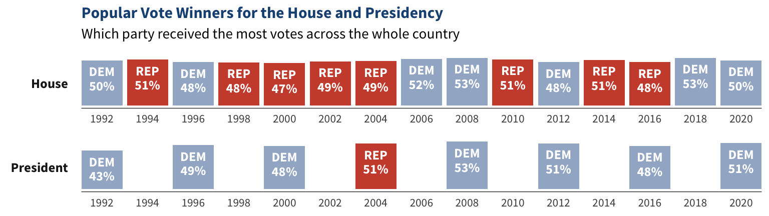